Course
Intermediate Python
4 hr
1.4M
When Wes McKinney started writing pandas, he had a rule of thumb: for pandas to work optimally, the machine’s RAM size must be 5–10 times larger than the dataset in question. This rule was easy to follow around 2010, but now it is 2023.
By 2020, real-world datasets had already grown to sizes that could easily crash everyday laptops and machines. Anticipating this problem well in advance, a solution was released in 2015.
Dask is an open-source library developed by the creators of Anaconda to tackle the challenges of scalable and efficient computing on large datasets that exceed the memory capacity of a single machine.
This tutorial provides a comprehensive introduction to Dask and its crucial features, including interfaces for DataFrames, Arrays, and Bags.
Like any other library, you can install Dask in three ways: Conda, Pip, and from source.
Since this is an introductory article on Dask, we won’t cover the last installation method, as it is for maintainers.
If you use Anaconda, Dask is included in your default installation (which is a mark of how popular the library is). If you wish to reinstall or upgrade it, you can use the install command:
conda install daskThe PIP alternative is the following:
pip install "dask[complete]"Adding the [complete] extension also installs the required dependencies of Dask, eliminating the need to install NumPy, Pandas, and Tornado manually.
You can check if the installation was successful by looking at the library version:
import dask

dask.__version__
Output:
'2023.5.0'Most of your Dask work will be focused on three interfaces: Dask DataFrames, Arrays, and Bags. Let’s import them along with numpy and pandas to use for the rest of the article:
import dask.array as da
import dask.bag as db
import dask.dataframe as dd
import numpy as np
import pandas as pdOn a high-level, you can think of Dask as a wrapper that extends the capabilities of traditional tools like pandas, NumPy, and Spark to handle larger-than-memory datasets.
When faced with large objects like larger-than-memory arrays (vectors) or matrices (dataframes), Dask breaks them up into chunks, also called partitions.
For example, consider the array of 12 random numbers in both NumPy and Dask:
narr = np.random.rand(12)

narr
array([0.9261154 , 0.87774082, 0.87078873, 0.22309476, 0.24575174,
0.04182393, 0.31476305, 0.04599283, 0.62354124, 0.97597454,
0.23923457, 0.81201211])darr = da.from_array(narr, chunks=3)
darr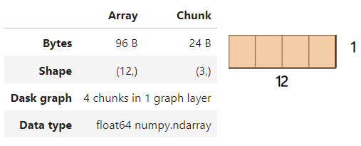
The image above shows that the Dask array contains four chunks as we set chunks to 3. Under the hood, each chunk is a NumPy array in itself.
Now, let’s consider a much larger example. We will create two 10k by 100k arrays (1 billion elements) and perform element-wise multiplication in both libraries while measuring the performance:
# Create the NumPy arrays
arr1 = np.random.rand(10_000, 100_000)
arr2 = np.random.rand(10_000, 100_000)

# Create the Dask arrays
darr1 = da.from_array(arr1, chunks=(1_000, 10_000))
darr2 = da.from_array(arr2, chunks=(1_000, 10_000))
%%time
result_np = np.multiply(arr1, arr2)Wall time: 3.19 s%%time
result_dask = da.multiply(darr1, darr2)Wall time: 94.8 msThe above code demonstrates the element-wise multiplication of two large arrays using both NumPy and Dask. As shown in the output, Dask is approximately 34 times faster than NumPy for this computation. The performance gains become even more significant as the computation and array size increase.
Dask uses a similar approach of chunking and distributing these chunks across all available cores on your machine for other objects as well.
To fully appreciate the benefits of Dask, we need a large dataset, preferably over 1 GB in size. However, downloading such a dataset to follow along in the tutorial may not be optimal. Instead, you can use this script, which generates a synthetic dataset with 10 million rows, 10 numeric features, and 10 categorical features.
Please ensure that your machine has at least 12 GB of RAM to run the script.
Once you have the large_dataset.csv file in your workspace, you can load it using the read_csv function from the Dask DataFrames interface (dd):
import dask.dataframe as dd

dask_df = dd.read_csv("data/large_dataset.csv")

dask_df.head()
Even though the file is large, you will notice that the result is fetched almost instantaneously. For even larger files, you can specify the `blocksize` parameter, which determines the number of bytes to break up the file into.
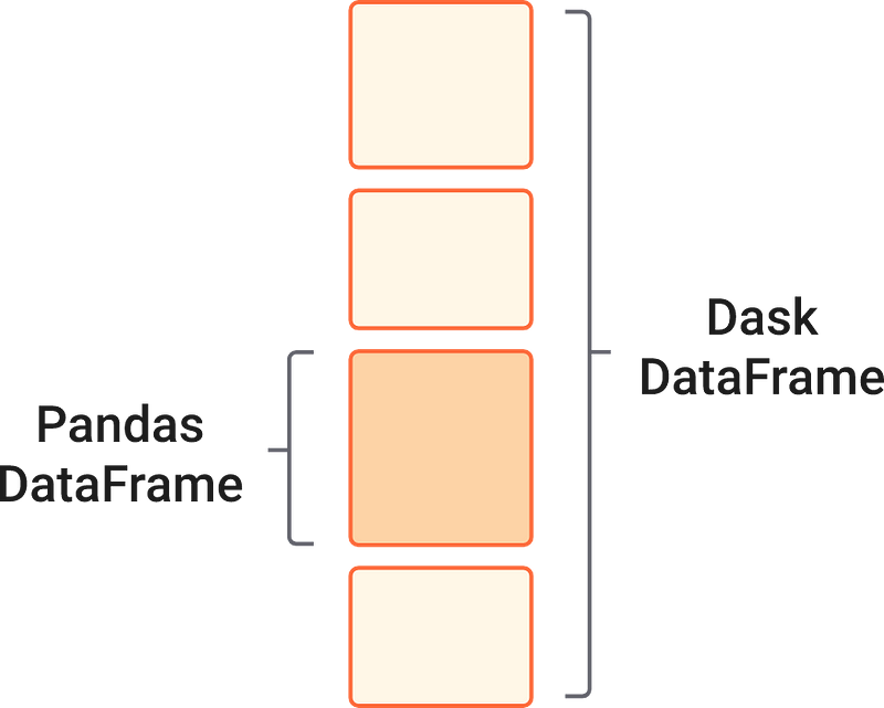
Similar to how Dask Arrays contain chunks of small NumPy arrays, Dask is designed to handle multiple small Pandas DataFrames arranged along the row index.
As you might guess from the read_csv function, most of the commonly used syntax and functionality of the pandas API is preserved in Dask. The following code blocks should be familiar to you from your time working with pandas.
In this example, we're doing some pretty straightforward column operations on our Dask DataFrame, called dask_df. We're adding the values from the column Numeric_0 to the result of multiplying the values from Numeric_9 and Numeric_3. We store the outcome in a variable named result.
result = (
   dask_df["Numeric_0"] + dask_df["Numeric_9"] * dask_df["Numeric_3"]
)

result.compute().head()


0    1.301960
1    1.190679
2    1.100955
3    0.758272
4    0.926729
dtype: float64
As we’ve mentioned, Dask is a bit different from traditional computing tools in that it doesn't immediately execute these operations. Instead, it creates a kind of 'plan' called a task graph to carry out these operations later on. This approach allows Dask to optimize the computations and parallelize them when needed. The compute() function triggers Dask to finally perform these computations, and head() just shows us the first few rows of the result.
Now, let's look at how Dask can filter data. We're selecting rows from our DataFrame where the value in the "Categorical_5" column is "A".
This filtering process is similar to how you'd do it in pandas, but with a twist - Dask does this operation lazily. It prepares the task graph for this operation but waits to execute it until we call compute(). When we run head(), we get to see the first few rows of our filtered DataFrame.
dask_df[dask_df["Categorical_5"] == "A"].compute().head()
Next, we're going to generate some common summary statistics using Dask's describe() function.
It gives us a handful of descriptive statistics for our DataFrame, including the mean, standard deviation, minimum, maximum, and so on. As with our previous examples, Dask prepares the task graph for this operation when we call describe(), but it waits to execute it until we call compute().
dask_df.describe().compute()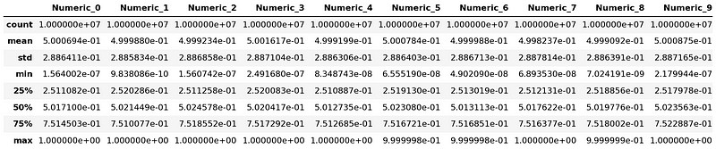
dask_df["Categorical_3"].value_counts().compute().head()Categorical_3
O 386038
C 385804
A 385493
P 385490
K 385116
Name: count, dtype: int64We also use value_counts() to count the number of occurrences of each unique value in the "Categorical_3" column. We trigger the operation with compute(), and head() shows us the most common values.
Finally, let's use the groupby() function to group our data based on values in the "Categorical_8" column. Then we select the "Numeric_7" column and calculate the mean for each group.
This is similar to how you might use ‘groupby()’ in pandas, but as you might have guessed, Dask does this lazily. We trigger the operation with compute(), and head() displays the average of the "Numeric_7" column for the first few groups.
dask_df.groupby("Categorical_8")["Numeric_7"].mean().compute().head()


Categorical_8
A    0.498497
B    0.499767
C    0.500622
D    0.500307
E    0.499530
Name: Numeric_7, dtype: float64
Check out this section of Dask user guide on the rest of the familiarities between pandas and Dask.
Now, let’s explore the use of the compute function at the end of each code block.
Dask evaluates code blocks in lazy mode compared to Pandas’ eager mode, which returns results immediately.
To draw a parallel in cooking, lazy evaluation is like preparing ingredients and chopping vegetables in advance but only combining them to cook when needed. The compute function serves that purpose.
In contrast, eager evaluation is like throwing ingredients into the fire to cook as soon as they are ready. This approach ensures everything is ready to serve at once.
Lazy evaluation is key to Dask’s excellent performance as it provides:
compute is called), avoiding unnecessary intermediate results that may not be used in the final result.When the results of compute are returned, they are given as Pandas Series/DataFrames or NumPy arrays instead of native Dask DataFrames.
>>> type(dask_df)
dask.dataframe.core.DataFrame


>>> type(
   dask_df[["Numeric_5", "Numeric_6", "Numeric_7"]].mean().compute()
)

pandas.core.series.Series
The reason for this is that most data manipulation operations return only a subset of the original dataframe, taking up much smaller space. So, there won’t be any need to use parallelism of Dask, and you continue the rest of your workflow either in pandas or NumPy.
Dask Bags and Dask Delayed are two components of the Dask library that provide powerful tools for working with unstructured or semi-structured data and enabling lazy evaluation.
While in the past, tabular data was the most common, today’s datasets often involve unstructured files such as images, text files, videos, and audio. Dask Bags provides the functionality and API to handle such unstructured files in a parallel and scalable manner.
For example, let’s consider a simple illustration:
import dask.bag as db

# Create a Dask Bag from a list of strings
b = db.from_sequence(["apple", "banana", "orange", "grape", "kiwi"])

# Filter the strings that start with the letter 'a'
filtered_strings = b.filter(lambda x: x.startswith("a"))

# Map a function to convert each string to uppercase
uppercase_strings = filtered_strings.map(lambda x: x.upper())

# Compute the result as a list
result = uppercase_strings.compute()

print(result)
['APPLE']
In this example, we create a Dask Bag b from a list of strings. We then apply operations on the Bag to filter the strings that start with the letter 'a' and convert them to uppercase using the filter() and map() functions, respectively. Finally, we compute the result as a list using the compute() method and print the output.
Now imagine that you can perform even more complex operations on billions of similar strings stored in a text file. Without the lazy evaluation and parallelism offered by Dask Bags, you would face significant challenges. (Read more about Bags in the Dask documentation).
As for Dask Delayed, it provides even more flexibility and introduces lazy evaluation and parallelism to various other scenarios. With Dask Delayed, you can convert any native Python function into a lazy object using the @dask.delayed decorator.
Here is a simple example:
%%time

import time
import dask


@dask.delayed
def process_data(x):
   # Simulate some computation
   time.sleep(1)
   return x**2


# Generate a list of inputs
inputs = range(1000)

# Apply the delayed function to each input
results = [process_data(x) for x in inputs]

# Compute the results in parallel
computed_results = dask.compute(*results)


Wall time: 42.1 s
In this example, we define a function process_data decorated with @dask.delayed. The function simulates some computational work by sleeping for 1 second and then returning the square of the input value.
Without parallelism, performing this computation on 1000 inputs would have taken more than 1000 seconds. However, with Dask Delayed and parallel execution, the computation only took about 42.1 seconds.
This example demonstrates the power of parallelism in reducing computation time by efficiently distributing the workload across multiple cores or workers.
That’s what parallelism is all about.
Dask is one of the cornerstone libraries in the data ecosystem. It extends the functionality of most of the beloved libraries like NumPy, Pandas, and Spark, allowing seamless handling of larger-than-memory datasets.
With Dask Bags and Dask delayed, it brings parallelism and lazy evaluation to untraditional scenarios like working with unstructured data or with native Python objects.
For the nitty-gritty details, be sure to give the Dask docs a thorough read.
If you are looking for a comprehensive resource on mastering Dask, check out our course, Parallel Programming With Dask in Python.
Start your Dask Journey Today!
Course
Course
Course
blog
Alex Castrounis
13 min
blog
Olivia van Aalst
3 min
cheat-sheet
Karlijn Willems
Tutorial
Kurtis Pykes
Tutorial
Bex Tuychiev
code-along
Filip Schouwenaars