Course
Introduction to R
4 hr
3M
Relational Operators or also known as comparators which help you see how one R-Object relates to another R-object. For example, you can check whether two objects are equal or not, which can be accomplished with the help of ==(double equal) sign. A logical operator which is TRUE on both sides, will return a logical value as TRUE since TRUE equals TRUE, as shown below.
TRUE == TRUE
TRUE
However, if you have TRUE on one side and FALSE on the other, you will get a logical value FALSE as an output.
TRUE == FALSE
FALSE
Apart from logical variables, you can check the equality of other types.
Let's compare strings and numbers.
100 == 100
TRUE
100 == 200
FALSE
'tutorial' == 'R'
FALSE
inequality operator, which is given by !- sign (a combination of exclamation followed by equal to).Now all the conditions which resulted in FALSE earlier, will turn TRUE, let's check it out!
100 != 200
TRUE
'tutorial' != 'R'
TRUE
TRUE != FALSE
TRUE
Similarly, the inequality operator can also be used for numerical and other R-Objects like matrices, vectors, and lists.
What if you want to check whether given two R-Objects which one of them is greater or less than the other. Well, of course, you can, using simple < and > sign (less-than and greater-than sign).
Let's first see a numerical example.
2 > 10
FALSE
-200 < 0
TRUE
As you can see, it is self-explanatory why $2$ is not greater than $10$ or why $-200$ is less than $0$. But, what about strings or characters? Let's see how it can be achieved.
It looks like R gives preference to alphabetical order while deciding which string or character is greater than the other.
In the example below, as t comes after R as per the alphabetical order; hence, t is greater than R.
'tutorial' > 'RRRRRRRRR'
TRUE
It is important to note that in R and almost all programming languages, TRUE is numerically interpreted as 1 and FALSE as 0. So based on this analogy, TRUE will be greater than FALSE.
TRUE > FALSE
TRUE
(>=) (or less than or equal to <=) another R-object. To achieve this, you can use the less than or equal to sign in combination with an equal sign. This means that if one of the two conditions (less than or equal to / greater than or equal to) is TRUE, then the complete condition will be TRUE.5 >= 5 # 5 is not greater than 5 but is equal, hence, it returns TRUE.
TRUE
5 >= 10
FALSE
You can learn about R data types in this DataCamp tutorial. It shows that R is pretty good with handling lists, matrices, and vectors.
So can the R comparators handle the R vectors? Let's find out.
For example, you have a row-vector that has a record of the number of views you got on your recent datacamp tutorial in the last 10 days. Now, you want to find out which days you received more than or equal to 100 views. You can use the greater-than sign off-the-shelf.
datacamp_views <- c(100,20,5,200,60,88,190,33,290,64)
length(datacamp_views)
10
datacamp_views >= 100
As you can see from the above output, for the first, fourth, seventh, and ninth, the results are TRUE, which on these days, the views were more than or equal to 100.
Similarly, you can also compare two vectors or even two matrices.
youtube_views <- c(10,20,1000,64,100,9,19,3,90,4)
So with this way, you can build a nice and simple application to find out when were your datacamp tutorial views more than your youtube video views or vice-versa.
How this works in R is that it compares the two vectors element-wise. For example, in the below output, if you consider the first element from both the vectors, you can see that the DataCamp views vector has a value of 100, which the other vector has a value 10, and hence, it returned TRUE.
datacamp_views > youtube_views
Let's quickly compare to numerics. If you remember elementary mathematics, there is a rule known as BODMAS (or PEMDAS), which means bracket of division, multiplication, addition, and subtraction based on which any mathematical equation is solved. So, you will use the same rule to solve the below two R expressions.
-6 * 5 + 2 >= -10 + 1 #on left hand side multiplication will be done first and then addition as per BODMAS
FALSE
More than 10 million people learn Python, R, SQL, and other tech skills using our hands-on courses crafted by industry experts.

R's ability to deal with different data structures for comparisons does not stop at vectors. Matrices and relational operators also work together seamlessly!
Instead of vectors (as in the previous example), the DataCamp and YouTube data are now stored in a matrix called views. The first row contains the DataCamp information; the second row the YouTube information. You will use R's inbuilt matrix function to create a matrix with the help of datacamp and youtube vectors created in the previous example.
datacamp_views <- c(100,20,5,200,60,88,190,33,290,64)
youtube_views <- c(10,20,1000,64,100,9,19,3,90,4)
views <- matrix(c(datacamp_views, youtube_views), nrow = 2, byrow = TRUE)
views
| 100 | 20 | 5 | 200 | 60 | 88 | 190 | 33 | 290 | 64 |
| 10 | 20 | 1000 | 64 | 100 | 9 | 19 | 3 | 90 | 4 |
Let's find out when were the views of both datacamp as well as youtube equal to 20.
views == 20
| FALSE | TRUE | FALSE | FALSE | FALSE | FALSE | FALSE | FALSE | FALSE | FALSE |
| FALSE | TRUE | FALSE | FALSE | FALSE | FALSE | FALSE | FALSE | FALSE | FALSE |
Great! So you are done with understanding how relational operators work, now let's move on to logical operators.
R helps you in combining the results of relational operators by providing you following logical operators:
AND ( & ) operatorOR ( | ) operatorNOT ( ! ) operatorLet's have a look at each one of them.

Let's look at some of the self-explanatory examples.
TRUE & TRUE # 1.1 = 1
TRUE
TRUE & FALSE # 1.0 = 0
FALSE
FALSE & FALSE # 0.0 = 0
FALSE
FALSE & TRUE # 0.1 = 0
FALSE
Similarly, instead of using logical values as above, you can use the results of comparators with these operators.
x <- 100
x < 200 & x >= 100 # since x is less than 200 but less than equal to 100, so it returns TRUE.
TRUE
x < 200 & x > 100 # this holds FALSE since the second comparison i.e. x greater than 100 is false.
FALSE
Let's look at some of the self-explanatory examples.
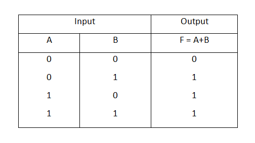
TRUE | TRUE # 1 + 1 = 1
TRUE
TRUE | FALSE # 1 + 0 = 0
TRUE
FALSE | FALSE # 0 + 0 = 0
FALSE
FALSE | TRUE # 0 + 1 = 0
TRUE
Let us use the same numerical example as used above, but this time the result should differ.
x <- 100
x < 200 | x > 100 # this holds TRUE since the first comparison i.e. x less than 100 is True.
TRUE
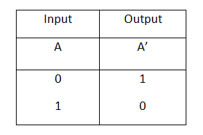
Let's look at some examples!
a = 1
!a # this returns false since not of a will be 0 which is FALSE.
FALSE
a = 0
!a #similar to the above example this return TRUE since a = 0 and not of a is 1.
TRUE
Let's look at some cases where the NOT operator can be helpful when dealing with R's in-built functions.
is.numeric(5) #returns TRUE since 5 is numeric
TRUE
!is.numeric(5) #not of the same will return FALSE
FALSE
is.numeric('aditya')
FALSE
The below example can be useful in a situation where you are dealing with a mix of numeric and string data, and you want to filter out the strings/characters from maybe a list and only keep numeric data.
!is.numeric('aditya')
TRUE
Finally, let's find out how logical operators function on vectors and matrices.
a <- c(FALSE, TRUE, FALSE)
b <- c(TRUE, TRUE, FALSE)
a & b # AND operator
a | b # OR operator
Based on the above two outputs, it is apparent that similar to vectors in relational operators. Logical operators also perform operations element-wise.
However, the NOT operator can only be applied on a single vector at a time or maybe on the result of two vectors.
!a
!b
In the example below, the NOT operator is outside the brackets, which means it is applied to the result of a and b. The below operator can also be termed as a NOR (Not-OR) operator.
!(a | b) # NOR operator
Before moving on to conditional statements, let's do a small exercise.
You have the same datacamp tutorial views in a vector form that you had defined above. Let's extract the last element from it using R's tail method.
last <- tail(datacamp_views,1)
print (last)
[1] 64
Let's find out if the last element is under 100 or above 100.
last < 100 | last > 100
TRUE
Since the last element is under 100, one of the expression satisfies that, hence, it returned TRUE.
Let's move on to the final topic of this tutorial, i.e., conditional statements!
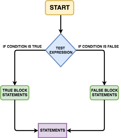
Until now, you have already learned about relational operators, which tells you how R-Objects relate to each other and logical operators, which allow you to combine logical values. R provides you a way to combine all of these operators and use the result to change the behavior of your R scripts. With this, let's get into the if and else statements.
The syntax of the if condition is defined below: if(condition){ // expression } The if statement takes an input a condition ( inside parentheses ) which you can relate to a relational or some logical operator and if that condition is TRUE then the R code associated with the condition ( inside curly brackets ) is executed. Simple, isn't it?
Let's understand it with an example.
Suppose you have a variable x which equals to -10, now, you will put a condition which checks whether x is greater than zero and negates that with a NOT operator. Since the condition is TRUE, the R code inside the curly brackets will be executed.
x <- -10
if (!x > 0){
    print("x is a negative number")
}
[1] "x is a negative number"
However, if you remove the NOT operator, then the condition will turn FALSE, and the code inside the curly brackets will not be executed.
if (x > 0){
    print("x is a positive number")
}
Let's now understand the else statement with the help of a syntax. if(condition){ // expression1 }else{ // expression2 } Unlike the if statement, the else statement does not require an explicit condition with it, it has to be used in combination with the if statement. The R code associated with the else statement is executed only if the condition of the if` statement is not TRUE.
Let's take the same if statement example to understand the else statement.
x <- -10
if (x > 0){
    print("x is a positive number")
}else{
    print("x is a negative number")
}
[1] "x is a negative number"
In the above example, since the if statement was not valid, hence, the else statement was executed.
Similar to if and else statement, you have else if statement which comes in between if and else statement. It is executed when the if statement condition is not satisfied. So, in short, the else statement is given the last priority. if(condition){ // expression1 }else if(condition){ // expression2 }else{ // expression3 }
x <- 0
if (x > 0){
    print("x is a positive number")
}else if (x == 0){
    print("x is zero")
}else{
    print("x is a negative number")
}
[1] "x is zero"
Predominantly, one of the reasons we use the else if statement is when the condition at hand is not mutually exclusive, meaning they could occur at the same time. Let's look at it with an example.
x <- 12
if (x %% 3 == 0){
    print("x is divisible by 3")
}else if (x %% 4 == 0){
    print("x is divisible by 4")
}else{
    print("x is neither divisible by 3 nor by 4")
}
[1] "x is divisible by 3"
In the above example, the if condition became TRUE, so R exits the control structure and does not go to the next statements even though the else if condition would evaluate to TRUE it didn't execute it. However, instead of else if statement if you would have used another if condition, then even that would have been executed.
Congratulations on finishing the tutorial.
This tutorial was a good starting point for beginners who are curious to learn the R programming language. As a good exercise, you might want to apply the relational and logical operators as conditions in the conditional statements.
There are still topics that are yet to be covered in R like Utilities in R and Machine Learning using R, which will be covered in the future tutorials, so stay tuned!
Please feel free to ask any questions related to this tutorial in the comments section below.
If you would like to learn more about R, take DataCamp's Intermediate R course.
Learn more about R
Course
Course
Course
Tutorial
DataCamp Team
Tutorial
Łukasz Deryło
Tutorial
Aditya Sharma
Tutorial
Carlo Fanara
Tutorial
Olivia Smith
Tutorial
Chloe Lubin