Course
Before we start with the introduction and learn about various data types in R, let's quickly set up the R environment both on the Terminal and Jupyter Notebook.
The following command is for Mac operating system, which will install R on your terminal.
brew install r --build-from-source
To verify the installation has been successful, just type R (upper-case) in the terminal, and you will enter into an R session, as shown below.
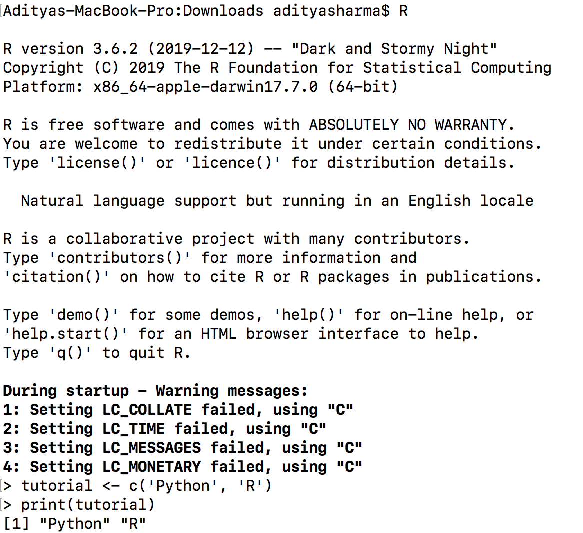
For installation on other operating systems, feel free to check this tutorial.
Now let's add R programming language as a kernel on jupyter notebook. Make sure you have jupyter notebook already installed on your system.
Go to your terminal and open the R session and enter the below two commands, which will add the R kernel to your jupyter notebook.
install.packages('IRkernel')
IRkernel::installspec()
Once the above two commands are successful, run jupyter from the terminal and open a notebook with R kernel as shown below:
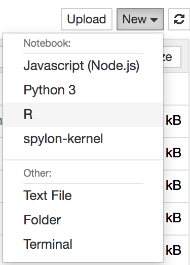
Now you are all set to write your first R code on jupyter notebook.
Introduction
To make use of R to the fullest, it is very important to know and understand various data types and data structures that exist in R and how they function. They play a key role in almost all problems and especially when you are working on machine learning problems, which are very data-centric.
In a programming language, we usually need variables to store information, which can be an integer, character, floating-point, boolean, etc. The type of the variable is purely based on which kind of information it holds. If it is assigned an integer, then the variable has a data type as int. Variables are merely reserved memory locations at which values are stored. As soon as you create a variable, some memory space is reserved for it.
Based on the data type of a variable, some memory will be allocated by the operating system. For example, in R programming, a variable that holds an integer will reserve a memory of 4 bytes and 1 byte for a character.
Programming languages like C, C++, and Java, variables are declared as data type; however, in Python and R, the variables are an object. Objects are nothing but a data structure having few attributes and methods which are applied to its attributes.
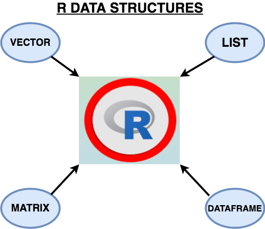
There are various kinds of R-objects or data structures which will be discussed in this tutorial like:
-
Vectors
-
Lists
-
Matrices
-
Arrays
-
Factors
Let's first understand some of the basic datatypes on which the R-objects are built like Numeric, Integer, Character, Factor, and Logical.
- Numeric: Numbers that have a decimal value or are a fraction in nature have a data type as numeric.
num <- 1.2
print(num)
[1] 1.2
You can check the data type of a using keyword class().
class(num)
'numeric'
- Integer: Numbers that do not contain decimal values have a data type as an integer. However, to create an integer data type, you explicitly use
as.integer()and pass the variable as an argument.
int <- as.integer(2.2)
print(int)
[1] 2
class(int)
'integer'
- Character: As the name suggests, it can be a letter or a combination of letters enclosed by quotes is considered as a character data type by R. It can be alphabets or numbers.
char <- "datacamp"
print(char)
[1] "datacamp"
class(char)
'character'
char <- "12345"
print(char)
[1] "12345"
class(char)
'character'
- Logical: A variable that can have a value of True and False like a boolean is called a logical variable.
log_true <- TRUE
print(log_true)
[1] TRUE
class(log_true)
'logical'
log_false <- FALSE
print(log_false)
[1] FALSE
class(log_false)
'logical'
- Factor: They are a data type that is used to refer to a qualitative relationship like colors, good & bad, course or movie ratings, etc. They are useful in statistical modeling.
To achieve this, you will make use of the c() function, which returns a vector (one-dimensional) by combining all the elements.
fac <- factor(c("good", "bad", "ugly","good", "bad", "ugly"))
print(fac)
[1] good bad  ugly good bad  ugly
Levels: bad good ugly
class(fac)
'factor'
The fac factor has three levels as good, bad, and ugly, which can be checked using the keyword levels, and the type of level will be a character.
levels(fac)
- 'bad'
- 'good'
- 'ugly'
nlevels(fac)
3
class(levels(fac))
'character'
Before moving forward, let us understand a couple of important tips that can come in handy!
- Always remember that R programming language is case-sensitive. All of the objects that are defined above should be used in the same manner, be it upper or lower, as shown in the example below.
Num
Error in eval(expr, envir, enclos): object 'Num' not found
Traceback:
- In R, you can check all the variables or objects that have been defined by you in the working environment by using keyword the
ls(), as shown below.
ls()
- 'char'
- 'int'
- 'num'
Lists

Unlike vectors, a list can contain elements of various data types and is often known as an ordered collection of values. It can contain vectors, functions, matrices, and even another list inside it (nested-list).
Lists in R are one-indexed, i.e., the index starts with one.
Let's understand the concept of lists with a quick example that will have three different types of data types stored in one list.
lis1 <- 1:5  # Integer Vector
lis1
- 1
- 2
- 3
- 4
- 5
lis2 <- factor(1:5)  # Factor Vector
lis2
- 1
- 2
- 3
- 4
- 5
Levels:
- '1'
- '2'
- '3'
- '4'
- '5'
lis3 <- letters[1:5]  # Character Vector
lis3
- 'a'
- 'b'
- 'c'
- 'd'
- 'e'
combined_list <- list(lis1, lis2, lis3)
combined_list
-
- 1
- 2
- 3
- 4
- 5
- 1
- 2
- 3
- 4
- 5
Levels:
- '1'
- '2'
- '3'
- '4'
- '5'
- 'a'
- 'b'
- 'c'
- 'd'
- 'e'
Let's access each vector in the list separately. To achieve this, you will use double square brackets since the three vectors are placed on one level inside the list. python
combined_list[[1]]
- 1
- 2
- 3
- 4
- 5
python
combined_list[[2]]
- 1
- 2
- 3
- 4
- 5
Levels:
- '1'
- '2'
- '3'
- '4'
- '5'
combined_list[[3]]
- 'a'
- 'b'
- 'c'
- 'd'
- 'e'
Now, let us try to access the fifth element from the third vector, which gives the letter e.
combined_list[[3]][5]
'e'
Finally, let's try to flatten the list. One important thing to remember is that since combined_list is a combination of character and numeric datatype, the character data type will get the precedence, and the data type of complete list will become a character.
flat_list <- unlist(combined_list)
class(flat_list)
'character'
flat_list
- '1'
- '2'
- '3'
- '4'
- '5'
- '1'
- '2'
- '3'
- '4'
- '5'
- 'a'
- 'b'
- 'c'
- 'd'
- 'e'
length(flat_list)
15
Vectors
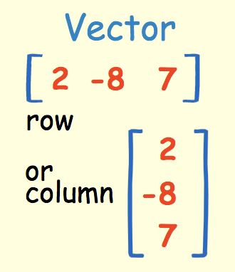
Vectors are an object which is used to store multiple information or values of the same data type. A vector can not have a combination of both integer and character. For example, if you want to store 100 students' total marks, instead of creating 100 different variables for each student, you would create a vector of length 100, which will store all the student marks in it.
A vector can be created with a function c(), which will combine all the elements and return a one-dimensional array.
Let's create a vector marks with data of five students of class numeric.
marks <- c(88,65,90,40,65)
class(marks)
'numeric'
Let us check the length of the vector, which should return the number of elements contained in it.
length(marks)
5
Now, let's try to access a specific element by its index.
marks[4]
40
marks[5]
65
marks[6] #returns NA since there is no sixth element in the vector
<NA>
-
Slicing: Similar to Python, the concept of slicing can be applied in R as well.
Let's try to access elements from second to fifth using slicing.
marks[2:5]
- 65
- 90
- 40
- 65
Let's now create a character vector that is similar to creating a numeric character.
char_vector <- c("a", "b", "c")
print(char_vector)
[1] "a" "b" "c"
class(char_vector)
'character'
length(char_vector)
3
char_vector[1:3]
- 'a'
- 'b'
- 'c'
If we create a vector that has both numeric and character values, the numeric values will get converted to a character data type.
char_num_vec <- c(1,2, "a")
char_num_vec
- '1'
- '2'
- 'a'
class(char_num_vec)
'character'
Let's create a vector with 1024 numeric values with the help of a slicing concept.
vec <- c(1:1024)
Now, try to access the middle and the last element. To do that, you will use the length function.
vec[length(vec)]
1024
vec[length(vec)/2]
512
- How do you create a vector of odd numbers?
To create a vector of odd numbers, you can use the function seq, which takes in three parameters: start, end, and step size.
seq(1,10, by = 2)
- 1
- 3
- 5
- 7
- 9
Matrix
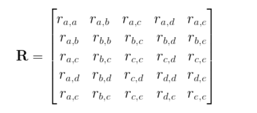
Similar to a vector, a matrix is used to store information about the same data type. However, unlike vectors, matrices are capable of holding two-dimensional information inside it.
The syntax of defining a matrix is:
M <- matrix(vector, nrow=r, ncol=c, byrow=FALSE, dimnames=list(char_vector_rownames, char_vector_colnames))
byrow=TRUE signifies that the matrix should be filled by rows. byrow=FALSE indicates that the matrix should be filled by columns (the default).
Let's quickly define a matrix M of shape $2\times3$.
M = matrix( c('AI','ML','DL','Tensorflow','Pytorch','Keras'), nrow = 2, ncol = 3, byrow = TRUE)
print(M)
     [,1]         [,2]      [,3]
[1,] "AI"         "ML"      "DL"
[2,] "Tensorflow" "Pytorch" "Keras"
Let's use the slicing concept and fetch elements from a row and column.
M[1:2,1:2] #the first dimension selects both rows while the second dimension will select
#elements from 1st and 2nd column
| AI | ML |
| Tensorflow | Pytorch |
DataFrame
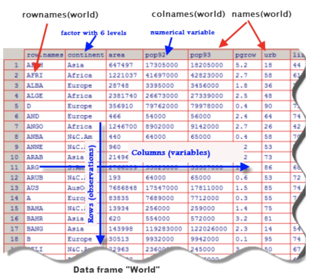
Unlike a matrix, Data frames are a more generalized form of a matrix. It contains data in a tabular fashion. The data in the data frame can be spread across various columns, having different data types. The first column can be a character while the second column can be an integer, and the third column can be logical.
The variables or features are in columnar fashion, also known as a header, while the observations are in rows with the first element being the name of the row followed by the actual data, also known as data rows.
DataFrame can be created using the data.frame() function.
DataFrame has been widely used in the reading comma-separated files (CSV), text files. Their use is not only limited to reading the data, but you can also use them for machine learning problems, especially when dealing with numerical data. DataFrames can be useful for understanding the data, data wrangling, plotting and visualizing.
Let's create a dummy dataset and learn some data frame specific functions.
dataset <- data.frame(
   Person = c("Aditya", "Ayush","Akshay"),
   Age = c(26, 26, 27),
   Weight = c(81,85, 90),
   Height = c(6,5.8,6.2),
   Salary = c(50000, 80000, 100000)
)
print(dataset)
  Person Age Weight Height Salary
1 Aditya  26     81    6.0  5e+04
2  Ayush  26     85    5.8  8e+04
3 Akshay  27     90    6.2  1e+05
class(dataset)
'data.frame'
nrow(dataset) # this will give you the number of rows that are there in the dataset dataframe
3
ncol(dataset) # this will give you the number of columns that are there in the dataset dataframe
5
df1 = rbind(dataset, dataset) # a row bind which will append the arguments in row fashion.
df1
| Person | Age | Weight | Height | Salary |
|---|---|---|---|---|
| <fct> | <dbl> | <dbl> | <dbl> | <dbl> |
| Aditya | 26 | 81 | 6.0 | 5e+04 |
| Ayush | 26 | 85 | 5.8 | 8e+04 |
| Akshay | 27 | 90 | 6.2 | 1e+05 |
| Aditya | 26 | 81 | 6.0 | 5e+04 |
| Ayush | 26 | 85 | 5.8 | 8e+04 |
| Akshay | 27 | 90 | 6.2 | 1e+05 |
df2 = cbind(dataset, dataset) # a column bind which will append the arguments in column fashion.
df2
| Person | Age | Weight | Height | Salary | Person | Age | Weight | Height | Salary |
|---|---|---|---|---|---|---|---|---|---|
| <fct> | <dbl> | <dbl> | <dbl> | <dbl> | <fct> | <dbl> | <dbl> | <dbl> | <dbl> |
| Aditya | 26 | 81 | 6.0 | 5e+04 | Aditya | 26 | 81 | 6.0 | 5e+04 |
| Ayush | 26 | 85 | 5.8 | 8e+04 | Ayush | 26 | 85 | 5.8 | 8e+04 |
| Akshay | 27 | 90 | 6.2 | 1e+05 | Akshay | 27 | 90 | 6.2 | 1e+05 |
Let's look at the head function which is very useful when you have millions of records and you want to look at only the first few rows of your data. Similarly, the tail function will output the last few rows of your data.
head(df1,3) # here only three rows will be printed
| Person | Age | Weight | Height | Salary | |
|---|---|---|---|---|---|
| <fct> | <dbl> | <dbl> | <dbl> | <dbl> | |
| 1 | Aditya | 26 | 81 | 6.0 | 5e+04 |
| 2 | Ayush | 26 | 85 | 5.8 | 8e+04 |
| 3 | Akshay | 27 | 90 | 6.2 | 1e+05 |
str(dataset) #this returns the individual class or data type information for each column.
'data.frame':    3 obs. of  5 variables:
 $ Person: Factor w/ 3 levels "Aditya","Akshay",..: 1 3 2
 $ Age   : num  26 26 27
 $ Weight: num  81 85 90
 $ Height: num  6 5.8 6.2
 $ Salary: num  5e+04 8e+04 1e+05
Now let's look at the summary() function, which comes in handy when you want to understand the statistics of your dataset. As shown below, it divides your data into three quartiles, based on which you can get some intuition about the distribution of your data. It also shows if there are any missing values in your dataset.
summary(dataset)
    Person       Age            Weight          Height        Salary
 Aditya:1   Min.   :26.00   Min.   :81.00   Min.   :5.8   Min.   : 50000
 Akshay:1   1st Qu.:26.00   1st Qu.:83.00   1st Qu.:5.9   1st Qu.: 65000
 Ayush :1   Median :26.00   Median :85.00   Median :6.0   Median : 80000
            Mean   :26.33   Mean   :85.33   Mean   :6.0   Mean   : 76667
            3rd Qu.:26.50   3rd Qu.:87.50   3rd Qu.:6.1   3rd Qu.: 90000
            Max.   :27.00   Max.   :90.00   Max.   :6.2   Max.   :100000
Conclusion
Congratulations on finishing the tutorial.
This tutorial was a good starting point for beginners who are curious to learn the R programming language. As a good exercise, feel free to check out more helper functions related to each data type.
There is a lot of information related to R that remains unraveled like Conditionals and Control Flow in R, Utilities in R, and the most exciting one Machine Learning using R, which will be covered in the future tutorials, so stay tuned!
Please feel free to ask any questions related to this tutorial in the comments section below.
If you would like to learn more about R, take DataCamp's Intermediate R course and check out the Introduction to Data frames in R tutorial.