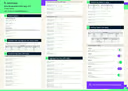
The data.table R package provides an enhanced version of data.frame that allows you to do blazing fast data manipulations. The data.table R package is being used in different fields such as finance and genomics and is especially useful for those of you that are working with large data sets (for example, 1GB to 100GB in RAM).
Although its typical syntax structure is not hard to master, it is unlike other things you might have seen in R. Hence the reason to create this cheat sheet. DataCamp’s data.table cheat sheet is a quick reference for doing data manipulations in R with the data.table R package and syntax
The cheat sheet will guide you from doing simple data manipulations using data.table’s basic i, j, by syntax, to chaining expressions, to using the famous set()-family.
Have this cheat sheet at your fingertips
Download PDFdata.table
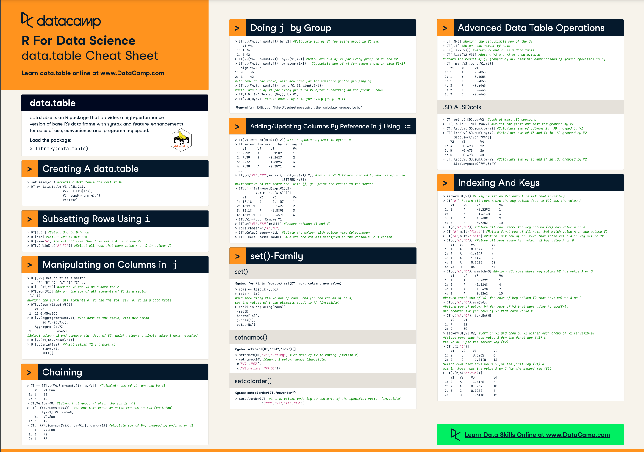
data.table is an R package that provides a high-performance version of base R’s data.frame with syntax and feature enhancements for ease of use, convenience and programming speed.
Load the Package:
library(data.table)Creating a data.table
> set.seed(45L) #Create a data.table and call it DT
> DT <- data.table(V1=c(1L,2L), V2=LETTERS[1:3], V3=round(rnorm(4),4), V4=1:12)
Subsetting Rows Using i
> DT[3:5,] #Select 3rd to 5th row
> DT[3:5] #Select 3rd to 5th row
> DT[V2=="A"] #Select all rows that have value A in column V2
> DT[V2 %in% c("A","C")] #Select all rows that have value A or C in column V2
Manipulating on columns in j
> DT[,V2] Return V2 as a vector
 [1] “A” “B” “C” “A” “B” “C” ...
> DT[,.(V2,V3)] #Return V2 and V3 as a data.table
> DT[,sum(V1)] #Return the sum of all elements of V1 in a vector
 [1] 18

#Return the sum of all elements of V1 and the std. dev. of V3 in a data.table
> DT[,.(sum(V1),sd(V3))]
    V1 V2
 1: 18 0.4546055

#The same as the above, with new names
> DT[,.(Aggregate=sum(V1), Sd.V3=sd(V3))]
    Aggregate Sd.V3
    1: 18        0.4546055

# Select column V2 and compute std. dev. of V3, which returns a single value & gets recycled
> DT[,.(V1,Sd.V3=sd(V3))]
#Print column V2 and plot V3
> DT[,.(print(V2), plot(V3), NULL)]
Chaining
#Calculate sum of V4, grouped by V1
> DT <- DT[,.(V4.Sum=sum(V4)), by=V1]
    V1   V4.Sum
 1: 1    36
 2: 2    42

#Select that group of which the sum is >40
> DT[V4.Sum>40]

#Select that group of which the sum is >40 (chaining)
> DT[,.(V4.Sum=sum(V4)), by=V1][V4.Sum>40]
    V1   V4.Sum
 1: 2    42

#Calculate sum of V4, grouped by ordered on V1
> DT[,.(V4.Sum=sum(V4)), by=V1][order(-V1)]
    V1   V4.Sum
 1: 2    42
 2: 1    36
Doing j by Group
#Calculate sum of V4 for every group in V1 Sum
> DT[,.(V4.Sum=sum(V4)),by=V1]
    V1 V4.
 1: 1 36
 2: 2 42

#Calculate sum of V4 for every group in V1 and V2
> DT[,.(V4.Sum=sum(V4)), by=.(V1,V2)]


#Calculate sum of V4 for every group in sign(V1-1)
> DT[,.(V4.Sum=sum(V4)), by=sign(V1-1)]
   sign V4.Sum
1: 0    36
2: 1    42

#The same as the above, with new name for the variable you’re grouping by
> DT[,.(V4.Sum=sum(V4)), by=.(V1.01=sign(V1-1))]

#Calculate sum of V4 for every group in V1 after subsetting on the first 5 rows
> DT[1:5,.(V4.Sum=sum(V4)), by=V1]
> DT[,.N,by=V1] #Count number of rows for every group in V1
Adding/Updating Columns by Reference in j using :=
> DT[,V1:=round(exp(V1),2)] #V1 is updated by what is after :=

> DT Return the result by calling DT
    V1      V2     V3          V4
 1: 2.72    A     -0.1107      1
 2: 7.39    B     -0.1427      2
 3: 2.72    C     -1.8893      3
 4: 7.39    A     -0.3571      4
 ...

#Columns V1 & V2 are updated by what is after :=
> DT[,c("V1","V2"):=list(round(exp(V1),2), LETTERS[4:6])]

#Alternative to the above one. With [], you print the result to the screen
> DT[,':='(V1=round(exp(V1),2), V2=LETTERS[4:6])][]

    V1       V2     V3         V4
 1: 15.18    D     -0.1107     1
 2: 1619.71  E     -0.1427     2
 3: 15.18    F     -1.8893     3
 4: 1619.71  D     -0.3571     4

# Remove V1
> DT[,V1:=NULL]

#Remove columns V1 and V2
> DT[,c("V1","V2"):=NULL]

#Delete the column with column name Cols.chosen
> Cols.chosen=c("A","B")
> DT[,Cols.Chosen:=NULL]

#Delete the columns specified in the variable Cols.chosen
> DT[,(Cols.Chosen):=NULL] set()-Family
set()
Syntax: for (i in from:to) set(DT, row, column, new value)
> rows <- list(3:4,5:6)
> cols <- 1:2

#Sequence along the values of rows, and for the values of cols,  set the values of those elements equal to NA (invisible)
> for(i in seq_along(rows))
 {set(DT,
 i=rows[[i]],
 j=cols[i],
 value=NA)}
setnames()
Syntax: setnames(DT,"old","new")[]
> setnames(DT,"V2","Rating") #Set name of V2 to Rating (invisible)
> setnames(DT, #Change 2 column names (invisible)
 c("V2","V3"),
 c("V2.rating","V3.DC"))
setcolorder()
Syntax: setcolorder(DT,"neworder")
#Change column ordering to contents of the specified vector (invisible)
> setcolorder(DT, c("V2","V1","V4","V3"))
Advanced Data Table Operations
> DT[.N-1] #Return the penultimate row of the DT
> DT[,.N] #Return the number of rows
> DT[,.(V2,V3)] #Return V2 and V3 as a data.table
> DT[,list(V2,V3)] #Return V2 and V3 as a data.table

#Return the result of j, grouped by all possible combinations of groups specified in by
> DT[,mean(V3),by=.(V1,V2)]
    V1    V2     V1
 1: 1     A      0.4053
 2: 1     B      0.4053
 3: 1     C      0.4053
 4: 2     A     -0.6443
 5: 2     B     -0.6443
 6: 2     C     -0.6443
.SD & SDCols
> DT[,print(.SD),by=V2] #Look at what .SD contains
> DT[,.SD[c(1,.N)],by=V2] #Select the first and last row grouped by V2
> DT[,lapply(.SD,sum),by=V2] #Calculate sum of columns in .SD grouped by V2

#Calculate sum of V3 and V4 in .SD grouped by V2
> DT[,lapply(.SD,sum),by=V2, .SDcols=c("V3","V4")]
    V2    V3        V4
 1: A     -0.478    22
 2: B     -0.478    26
 3: C     -0.478    30

#Calculate sum of V3 and V4 in .SD grouped by V2
> DT[,lapply(.SD,sum),by=V2, .SDcols=paste0("V",3:4)]
Indexing and Keys
> setkey(DT,V2) #A key is set on V2; output is returned invisibly
> DT["A"] #Return all rows where the key column (set to V2) has the value A
    V1     V2     V3          V4
 1: 1      A      -0.2392     1
 2: 2      A      -1.6148     4
 3: 1      A      1.0498      7
 4: 2      A      0.3262      10
> DT[c("A","C")] #Return all rows where the key column (V2) has value A or C
> DT["A",mult="first"] #Return first row of all rows that match value A in key column V2
> DT["A",mult="last"] #Return last row of all rows that match value A in key column V2

> DT[c("A","D")] #Return all rows where key column V2 has value A or D
    V1   V2    V3         V4
 1: 1    A    -0.2392     1
 2: 2    A    -1.6148     4
 3: 1    A     1.0498     7
 4: 2    A     0.3262     10
 5: NA   D     NA         NA

> DT[c("A","D"),nomatch=0] #Return all rows where key column V2 has value A or D
    V1     V2    V3           V4
 1: 1      A     -0.2392      1
 2: 2      A     -1.6148      4
 3: 1      A      1.0498      7
 4: 2      A      0.3262      10

#Return total sum of V4, for rows of key column V2 that have values A or C
> DT[c("A","C"),sum(V4)]

#Return sum of column V4 for rows of V2 that have value A, sum(V4), and another sum for rows of V2 that have value C
> DT[c("A","C"), by=.EACHI]
    V2     V1
 1: A      22
 2: C      30

#Sort by V1 and then by V2 within each group of V1 (invisible)
> setkey(DT,V1,V2)

#Select rows that have value 2 for the first key (V1) &  the value C for the second key (V2)
> DT[.(2,"C")]
    V1    V2    V3         V4
 1: 2     C     0.3262     6
 2: 2     C     -1.6148    12

# Select rows that have value 2 for the first key (V1) & within those rows the value A or C for the second key (V2)
> DT[.(2,c("A","C"))]
    V1   V2    V3          V4
 1: 2    A     -1.6148     4
 2: 2    A     0.3262      10
 3: 2    C     0.3262      6
 4: 2    C     -1.6148     12