Excel Power Pivot: A Step-by-Step Guide

Analyzing large Excel files often leads to sluggish performance. 

Power Pivot offers a different approach. It connects tables and handles calculations without compromising performance. Instead of fighting with VLOOKUP() chains and helper columns, you work with a structured system built directly into Excel.

In this guide, you'll learn how to set up data models, create table relationships, write DAX formulas, and build interactive reports using Power Pivot.

What Is Power Pivot And Why Is It Useful?

Power Pivot is Excel’s built-in data modeling engine. It lets you pull in larger datasets, connect multiple tables, and run complex calculations without the sluggishness you’d get from traditional worksheets.

How Power Pivot is different

Instead of storing data directly in a sheet, Power Pivot loads everything into Excel’s internal data model. 

A standard worksheet can reach roughly a million rows and usually slows down much earlier. Power Pivot bypasses that limit by compressing data and managing it separately, so you can work with tens of millions of rows while keeping workbook performance intact.

A relational structure instead of VLOOKUP chains

Once your data is in the model, you can relate tables using keys, just like a lightweight database. You don’t have to flatten everything into one giant sheet and use nested VLOOKUP() functions to force tables together. Power Pivot lets you analyze linked tables side by side, cleanly and reliably.

Stronger calculations with DAX

Power Pivot uses DAX (Data Analysis Expressions), a formula language explicitly built for analytical work. You can use this to create measures that go far beyond what a standard PivotTable can handle, from simple sums to time-based metrics, ratios, rolling windows, and other advanced calculations.

Example scenarios

Here are two examples of how businesses use Power Pivot in their work operations: 

• Sales performance tracking: Combine order history, product tables, and customer attributes, then build DAX measures for year-over-year revenue or customer lifetime value without manual merging.
• Operations reporting: Link inventory, shipments, and supplier data, then calculate fill rates, lead times, or forecast variances from the same model.

Simply put, Power Pivot gives you a database-style experience inside Excel. If you work with large or multi-table datasets, it can turn your messy reporting workflows into fast, scalable models you can build on.

Setting Up Power Pivot in Excel

Let's now see how you can start using Power Pivot in Excel. 

Enable Power Pivot

You don’t have to download Power Pivot. It’s already present in Excel. To enable it:

1. Open the Excel sheet 
2. Click on the Files from the ribbon
3. Select Options > Add-ins 
4. Then, select COM Add-ins from the drop-down and click Go
5. A pop-up window will appear. From here, choose Microsoft Power Pivot for Excel, then click OK

Now the Power Pivot will appear on your ribbon.

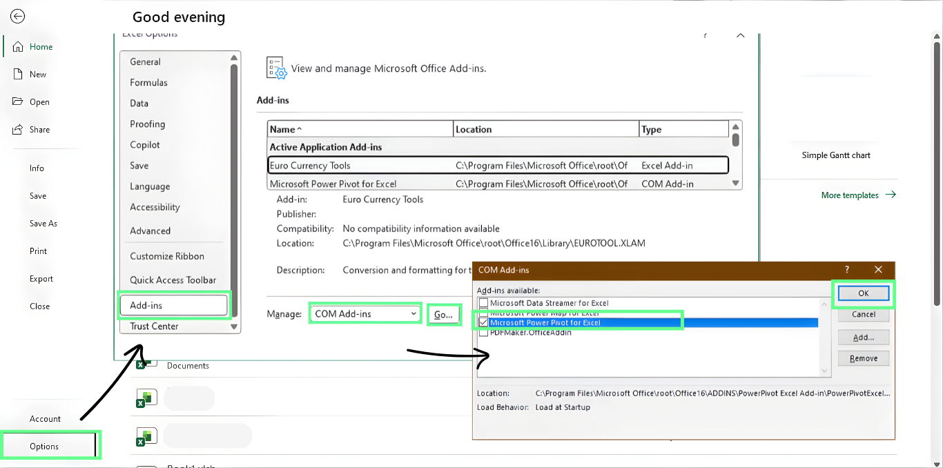
Enable the Power Pivot add-in in Excel. Image by Author.

Note: Power Pivot works only in Excel Professional Plus or Microsoft 365. If you do not see the tab after enabling it, the version of Excel on your computer might not include it.

Import data from multiple sources

You can now import data from different resources, such as an Excel file, a CSV file, or even a SQL Server database. 

For this example, we have two datasets in an .xlsb file:

1. sales.xlsb 

2. customer.xlsb 

To import them into Power Pivot:

1. Click on the Power Pivot tab and select Manage. A new window will open
2. Go to Home, then click Get External Data and choose From Other Sources
3. Scroll down and click the Excel File

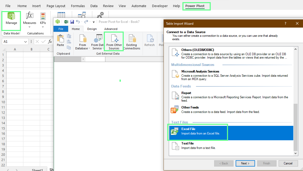
Get the data from other sources. Image by Author.

4. Now, in the pop-up, click Browse and select the customer.xlsb file 

5. Tick the Use first row as column header box and click Next

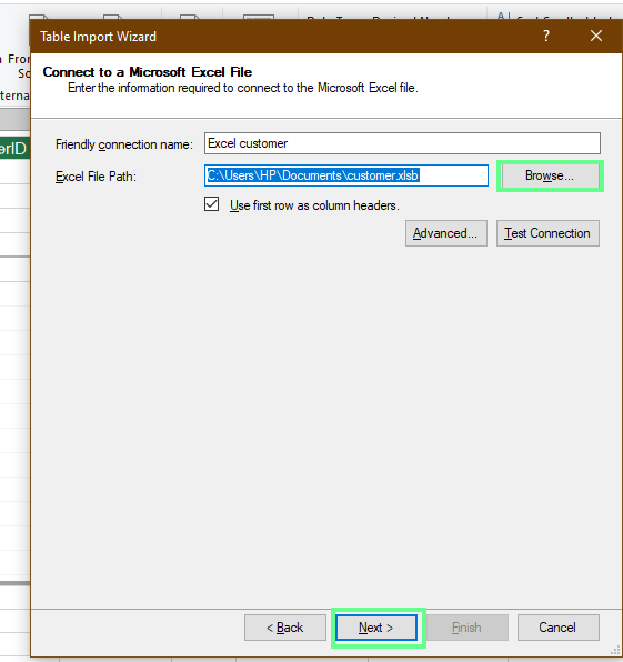
Import the Excel file into Power Pivot. Image by Author.

In the next window, click on Preview & Filter to see how your data will look before importing. Once satisfied, click OK, and it will show all rows have been successfully transferred. Then, click Close.

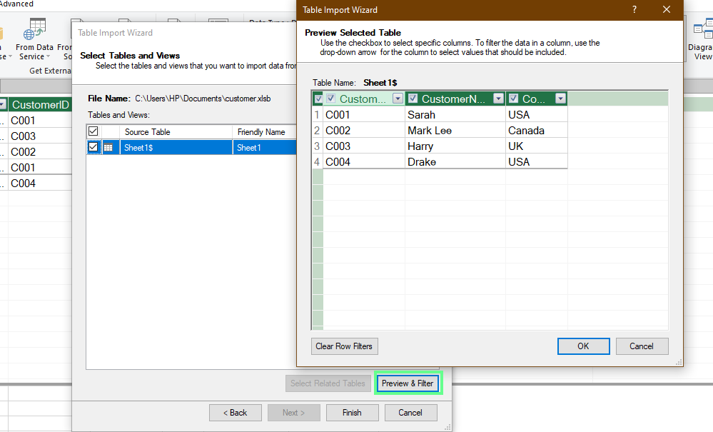
Preview the selected data. Image by Author. 

Repeat the same process for the sales.xlsb file. Then, at the bottom of the screen, both files will be shown as imported. Double-click on it and rename it. 

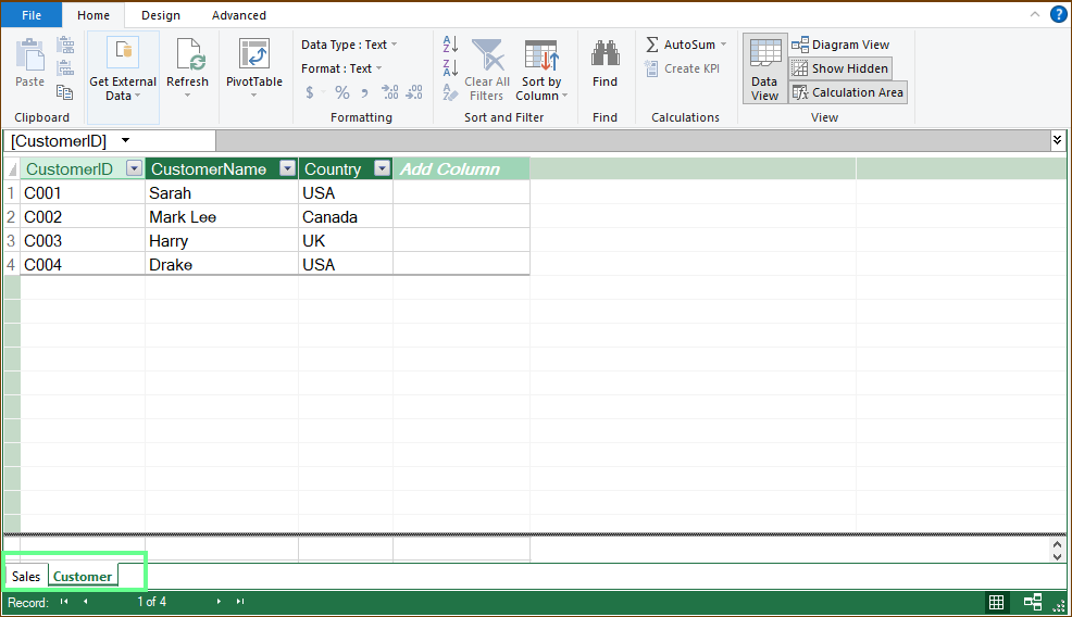
Both files imported. Image by Author.

Building Relationships And Data Models

Now that your data is loaded into Power Pivot, it’s time to link the tables so Excel understands how they connect. This step builds the foundation for all your reports.

Create relationships between tables

To create a relationship between the Sales and Customers table:

1. In the Home tab, click on the Diagram View. You’ll see both the imported tables there
2. Click CustomerID in the Sales table
3. Drag it to CustomerID in the Customer table to create a relationship between the two tables

Note: If you want to edit the relationship, right-click on the line and click Edit Relationship... In the window, select the columns you want to make the relation with.

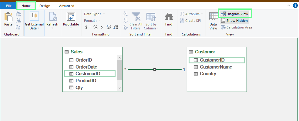
Build a relationship between the tables. Image by Author.

In this relationship, one customer can appear many times in the Sales table, but each customer appears only once in the Customers table. This is a simple one-to-many relationship that lets us use fields from both tables in PivotTables and do calculations without lookup formulas.

Design with a star schema

A star schema is one of the simplest ways to structure a Power Pivot model. It keeps your tables organized and makes calculations predictable.

First, you’ve to choose the fact table. In this case, Sales serves as the fact table because it holds the transactional records: date, customer, product, quantity, and amount.

Next, identify the dimension tables that describe the data in Sales. Some of its common examples include:

• Customers (primary key: CustomerID)
• Products (primary key: ProductID)
• Regions (primary key: RegionID)

Each dimension table has a primary key. You connect that key to the matching foreign key in the fact table:

• Customers.CustomerID → Sales.CustomerID
• Products.ProductID → Sales.ProductID
• Regions.RegionID → Customers.RegionID

Once linked, the Sales table sits at the center with dimension tables radiating around it. That’s your star. This structure keeps the model clear, speeds up calculations, and improves reporting consistency.

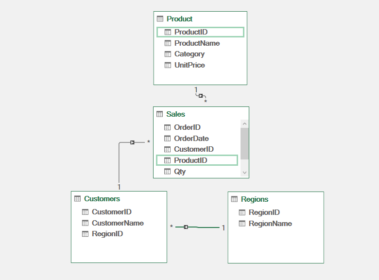
Create a star schema. Image by Author.

Add calculated columns

With your relationships in place, you can create new fields directly in the data model.

1. Switch to Data View

2. Select the empty Add Column field at the end of the table.

3. Input = [TotalAmount] / [Qty] and press Enter so Excel fills the entire column

4. Rename the header to PricePerUnit

This way, calculated columns become part of the table itself. They’re stored in the model, refreshed with your data, and stay available for any PivotTable or DAX measure you build later.

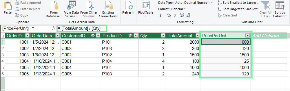
Add an extra calculated column. Image by Author.

Writing DAX Formulas For Analysis

Now that the model is ready, we can start creating DAX formulas to analyze the data. These formulas help us build totals, comparisons, and time-based calculations inside our reports.

Create measures

You should use measures when you want calculations that refresh automatically inside a PivotTable.

To create a measure:

1. Open the Power Pivot window

2. Go to Home > Calculations > New Measure

3. Enter a formula such as = SUM(Sales[TotalAmount])

4. Name it Total Sales and select OK

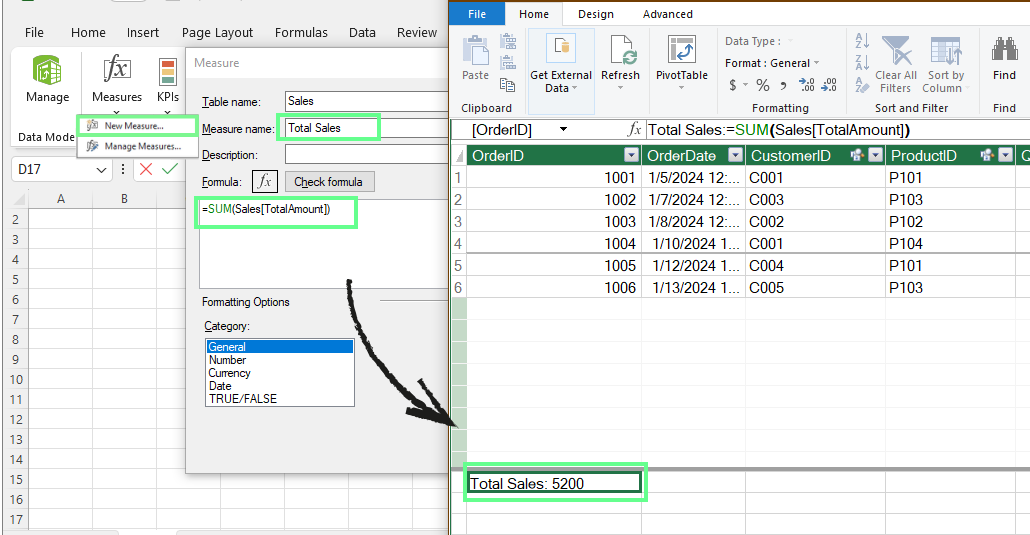
Create measures. Image by Author. 

Add a percent-of-total measure

You can also use this formula to add a percent of total measure:

= DIVIDE([Total Sales], CALCULATE([Total Sales], ALL(Regions)))

This would show each region’s share of overall revenue.

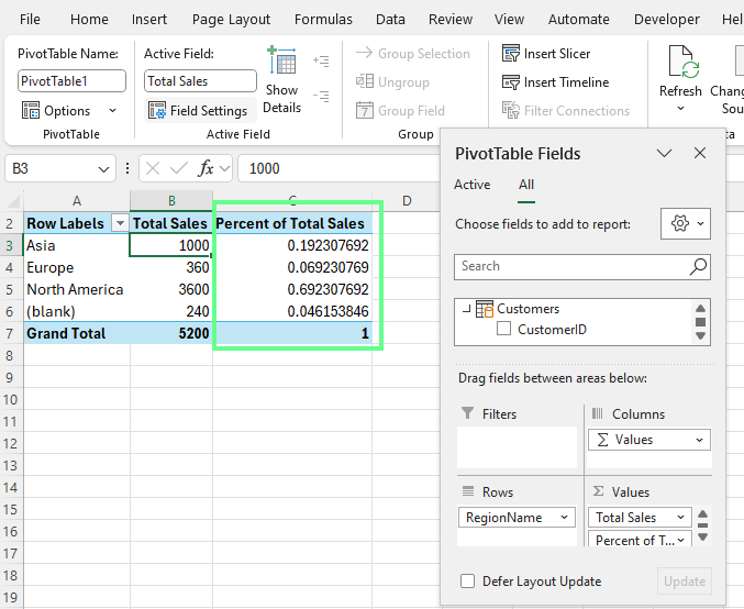
Add a percentage of the total measure. Image by Author.

Use time intelligence

Time intelligence functions are DAX formulas that understand how data moves across days, months, quarters, and years. They let you calculate year-to-date totals, compare results to prior periods, and evaluate trends without manually adjusting filters.

To see how these functions work in your model, you first need a proper Date table.

Set up the Date table

To set up the table: 

1. Go to Power Pivot > Add to Data Model
2. In Power Pivot, select the table and choose Design > Mark as Date Table

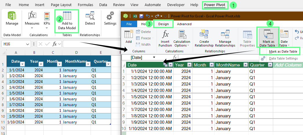
Create a data table. Image by Author.

3. Now from Home > Diagram View, relate Date[Date] → Sales[OrderDate].

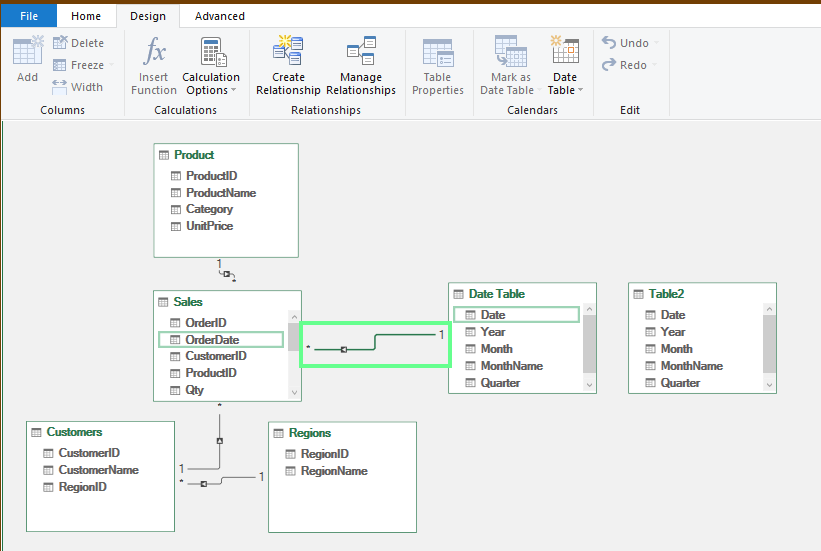
Link the Date Table[Date] to Sales[OrderDate]. Image by Author.

Create time intelligence measures

Once the Date table is done, you can build measures that evaluate performance across different periods.

Year-to-date:

Total Sales YTD :=
TOTALYTD([Total Sales], 'Date Table'[Date])

Last-year comparison:

Sales Last Year :=
CALCULATE([Total Sales], SAMEPERIODLASTYEAR('Date Table'[Date]))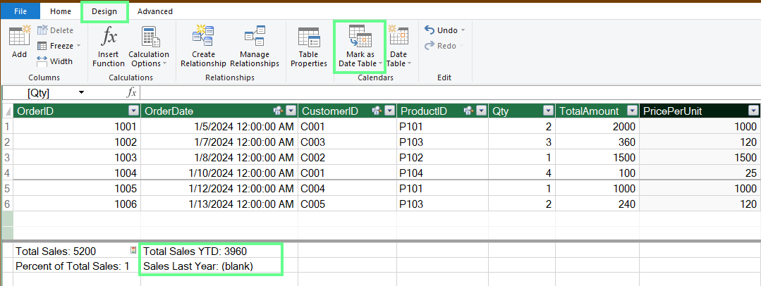

Calculate the time. Image by Author. 

With the measures ready, go back to Excel and create a PivotTable using the Data Model. Then, place fields from the Date table in the Rows area and add Total Sales, Total Sales YTD, and Sales Last Year into Values. 

This shows how the time intelligence measures work with the Date table inside the model.

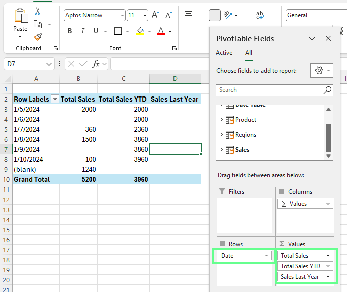
PivotTable showing Total Sales, YTD, and Last Year Date. Image by Author. 

Common DAX patterns

Some DAX formulas come up often because they help you break down data quickly and answer common questions. Here are two patterns that work well in many models:

Average per category:

Average Sales Per Category :=
AVERAGE(Sales[TotalAmount])

Running total across dates:

Running Total Sales :=
CALCULATE(
    [Total Sales],
    FILTER(ALL('Date'), 'Date'[Date] <= MAX('Date'[Date]))
)

When creating measures, make these few simple habits: 

• Name them clearly
• Keep formulas readable
• Use variables (VAR) when the measure gets long. 

It makes the model easier to understand when you go back to it later.

Visualizing And Interacting With Your Model

Now that the model and measures are done, let’s turn the data into visuals you can explore and adjust in real time.

Create PivotTables and PivotCharts

Here’s how to insert a PivotTable from the data model to work directly with your connected tables:

1. Open an Excel sheet
2. Go to Insert > PivotTable > From Data Model
3. Select New Worksheet

In the PivotTable Fields pane, you can now pull fields from any table. For example:

• Drag RegionName from the Regions table into Rows
• Drag Total Sales into Values

Because we built relationships earlier, Excel automatically brings everything together.

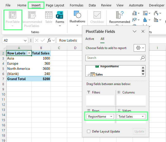
Create a PivotTable using the Power Pivot data. Image by Author.

If you want a visual, click anywhere inside the PivotTable, go to Insert > PivotChart, choose a chart type (like Clustered Column), and confirm. The chart stays linked to the PivotTable, so everything updates together.

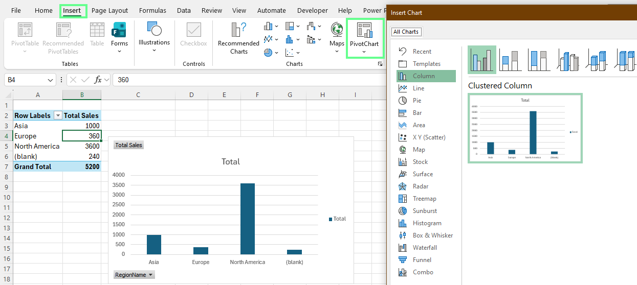
Add PivotChart. Image by Author.

Add slicers and filters

Slicers give you quick, button-style filters that make the report interactive. To add them:

1. Click on your Pivot table
2. Go to Insert > Slicer
3. Choose fields like RegionName or ProductName

A slicer appears as a box on the sheet. When you click different items, the PivotTable and chart update instantly. If you have multiple PivotTables, you can connect a single slicer to them all for consistent filtering across the page.

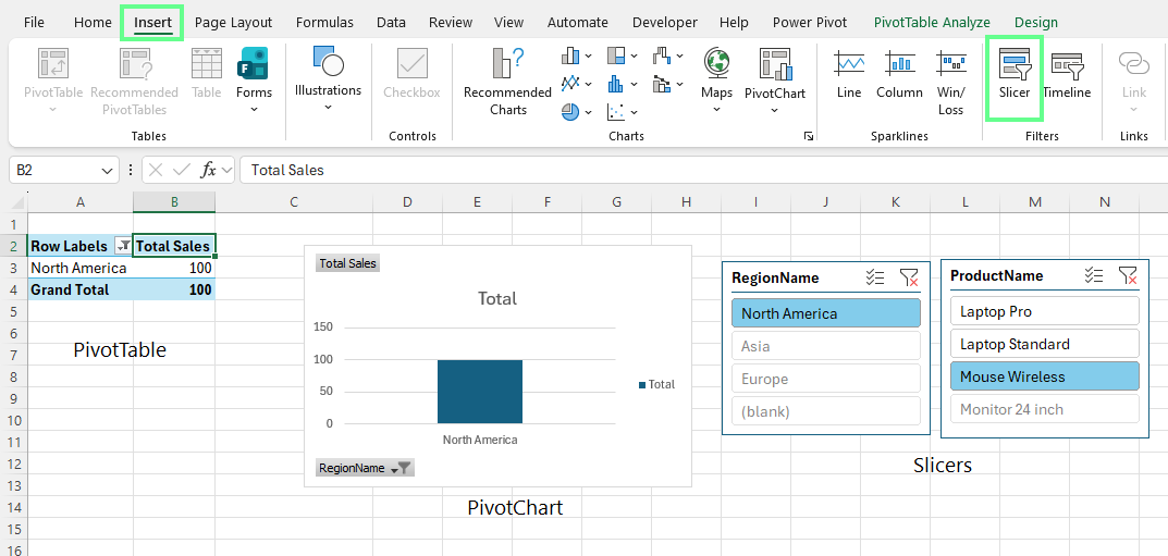
Add Slicers. Image by Author.

Build KPIs

KPIs help you see performance against a target without adding extra calculations to the sheet. To build yours:

1. In the Power Pivot window, go to KPIs > New KPI
2. Set Total Sales as the base measure
3. Use Absolute value, enter your target (for example, 4000), adjust thresholds, and pick an icon style
4. Click OK to create the KPI

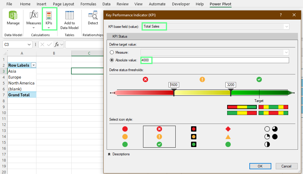
Set the KPI of a measure. Image by Author.

5. In the PivotTable fields pane, expand the Sales table, then expand the Total Sales
6. From there, drag the Total Sales and Status to the Value field

Now you can see the target performance against a threshold. 

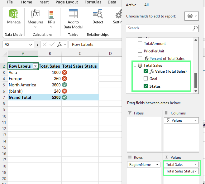
Display the KPI status in an Excel PivotTable. Image by Author.

Optimizing Power Pivot Performance

Once the model is built, we want to keep it fast and easy to work with. Power Pivot can handle large datasets, but a few minor adjustments help the file stay responsive, especially as you add more data over time.

Reduce model size

A lighter model runs faster, so remove anything you don’t need.

You can delete unused columns in Data View. Even if a column never appears in a PivotTable, it still takes memory, so trimming them keeps the model clean.

When you bring in new data, use Power Query to filter rows and columns before they enter the model. That way, only the fields you care about are loaded, which keeps everything cleaner.

Try to avoid calculated columns unless they’re required because they store a value for each row, which quickly increases file size. On the contrary, measures are more efficient because they calculate only when a PivotTable needs them. 

Choose efficient data types

Power Pivot compresses data differently depending on the data type. If you use the right type, it can make a noticeable difference.

In Data View, select a column and choose the most accurate type under Data Type on the ribbon. For example:

• Whole numbers > Whole Number
• Decimal values > Decimal Number
• IDs or codes that aren’t used for math > Text

When you choose the correct type, Power Pivot compresses the column better, which reduces size and speeds up calculations.

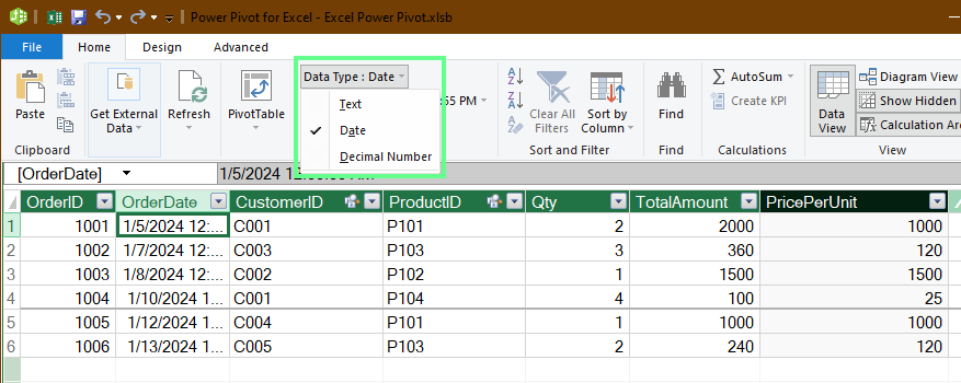
Check and use the correct data type. Image by Author.

Handle refresh and calculation issues

If your PivotTables don’t reflect the latest data, go to the Power Pivot tab and click Refresh All. This reloads everything from your source files.

When numbers look off, open Diagram View and check your relationships because a missing or broken relationship can cause totals to jump or filter incorrectly.

If you ever run into a DAX error, especially with more complex measures, it often means the formula is referencing itself indirectly. In this case, rewrite the measure with simpler logic or use VAR blocks to resolve the circular reference.

Integrating With Power Query And Power BI

One of the advantages of Power Pivot is how easily it works with the rest of the Microsoft data stack. We can use Power Query to clean and shape the data before it enters the model, or move the entire model into Power BI when you need interactive dashboards.

Clean and transform data in Power Query

Power Query is the best place to prepare your data before loading it into Power Pivot. It lets you clean, filter, and shape everything up front so the model stays organized.

You can open Power Query by going to Data > From Text/CSV > Transform. This brings the data into the editor, where you can:

• Remove duplicate rows
• Rename or reorder columns
• Filter out the values you don’t need
• Change data types before they reach the model

Power Query records each step on the right side of the window. That means the cleanup runs automatically whenever you refresh the file.

When everything looks right, select Close & Load To, then choose Data Model. The cleaned data loads directly into Power Pivot.

Export models to Power BI

You can also take your Power Pivot model into Power BI when you need richer visuals or shared dashboards. Here’s how:

1. Save your Excel workbook
2. Open Power BI Desktop
3. Go to Get Data > Excel Workbook
4. Select your file

Power BI imports the tables and relationships exactly as they exist in Power Pivot. From there, you can build dashboards, collaborate with your team, and set up scheduled refreshes so your reports stay up to date without manual steps.

Best Practices for Sustainable Models

As your model grows, keeping things organized makes it easier for you to update, debug, and build on it later. So, here are a few habits that help the model stay clean and reliable over time:

Naming conventions and organization

Clear names make a big difference when you come back to a file after weeks or months. That’s why you should use readable measure names like Total_Sales, Total_Quantity, or Profit_Margin so you always know what each measure represents.

You can also group related measures into Display Folders in the Power Pivot window. When the model gets larger, these folders make it easier to find the calculations you need.

Data validation

Before you trust the numbers, run a few quick checks:

• Compare totals from the source data with totals in your PivotTables
• Use simple DAX checks like:

• COUNTROWS() to confirm how many rows are in a table

• DISTINCTCOUNT() to verify unique values, such as customers or products

These small tests help you spot missing relationships, incorrect filters, or data issues before they cause bigger problems.

Maintain and update your models

When new data arrives, go to the Power Pivot tab and choose Refresh or Refresh All. As a result, Power Pivot reloads everything from the connected sources.

Before making major structural changes such as adding new relationships or rewriting key measures, save a backup copy of the file. It gives you a safe fallback if something doesn’t go as planned.

Final Thoughts

Power Pivot brings your data together in one place and helps you build reports that are clear and reliable. Once the model is set up, explore your numbers, create visuals, and update everything with a single refresh.

If you want to learn Excel’s full set of tools, check out our Data Analysis with Excel Power Tools track as well as our (of course) Power Pivot in Excel course.