VLOOKUP() Excel: What It Is and How to Use It

You’ve probably heard about VLOOKUP(). It’s one of the most well-known (if not the most well-known) function in Excel. And once you figure out how it works, you will love using it because it solves a notoriously tricky and time-consuming problem. VLOOKUP is really Microsoft’s way of giving you back a lot of time. 

In this article, I’ll demystify how VLOOKUP() works and walk you through its most common uses. And you can always come back to this article later if you forget one of the arguments. 

What Does VLOOKUP() Do?

Now that I’ve set the stage, let's get clear on what VLOOKUP() actually does. 

In essence, VLOOKUP() searches for a value in the first column of a table (or range of cells) and returns a value from another column in the same row. 

Think of it like this ask: "Find this item in my list, and give me something else from the same row."

There are four important arguments that you use every time: 

=VLOOKUP(lookup_value, table_array, col_index_num, [range_lookup])

• lookup_value: The value you want to search for.

• table_array: The range of cells containing your data (including both the column to search and the column(s) to return).

• col_index_num: The column number (starting from 1 for the leftmost) in the table_array from which to return the value.

• [range_lookup]: Optional. Enter FALSE for an exact match (this is usually what you want), or TRUE for an approximate match.

VLOOKUP() is a function where you have to understand that arguments. Not all functions are like this but VLOOKUP() definitely is. 

Excel VLOOKUP() Basic Example

Let’s put VLOOKUP() to work. Suppose you have a simple table of products and prices, like so: 

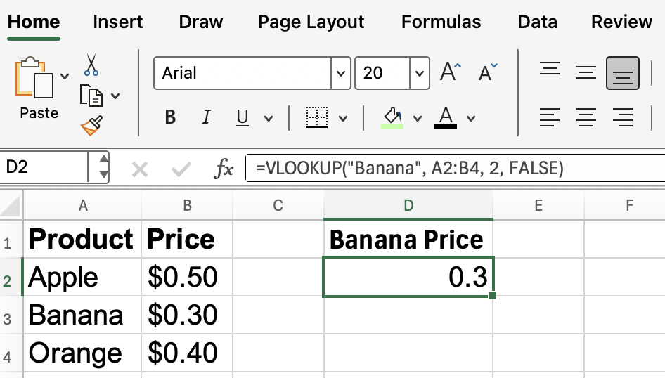
Say you want to know the price of a banana. You can use:

=VLOOKUP("Banana", A2:B4, 2, FALSE)

• "Banana" is the value you're searching for.

• A2:B4 is the data range.

• 2 tells Excel to return the value from the second column, which is Price.

• FALSE means you want an exact match. (More on this particular argument later. It’s the one that is the most confusing.)

This formula will return $0.30. 

Now, hard-coding the value isn’t always ideal, which brings us to our next point:

VLOOKUP() with Cell References Instead of Hard-Coding

In that last example, I hard-coded the lookup value. In practice, you'll often want to reference a cell. This makes your formula dynamic and reusable. For example, if you enter "Orange" in cell D2, you can use:

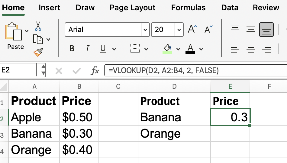
=VLOOKUP(D2, A2:B4, 2, FALSE)

Now, anytime you change the value in D2, the formula will fetch the corresponding price and you will discover that there is no need to edit the formula itself. 

VLOOKUP() Using Exact vs. Approximate Match

Now you might be wondering about that fourth argument, [range_lookup]. Sometimes, it doesn’t matter but other times it has a big impact on your results. The heuristic is that most of the time, you’ll want FALSE for an exact match.

• Use FALSE for things like names, IDs, or product codes where you need a precise match.

• Use TRUE for ranges (think like tax brackets or grading scales) where you want the closest value without going over. Just remember (and this is also important): your lookup column must be sorted in ascending order when using TRUE.

Let’s see an approximate match example:

Suppose you have this table for tax rates:

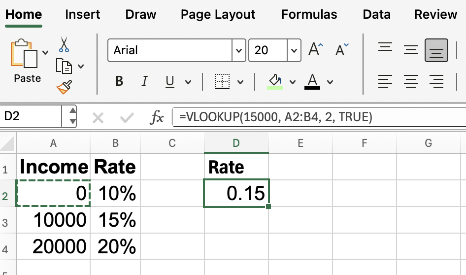
If your income is $15,000:

=VLOOKUP(15000, A2:B4, 2, TRUE)

Excel will find the closest value less than or equal to 15000 (which is 10000) and return 15%.

But again, for most lookups, though, stick with FALSE.

Common Pitfalls and Limitations

Like anything, VLOOKUP() has some limitations, so you don’t get tripped up later. Here are a few things to watch for:

• Only searches left-to-right. This is the big limitation that comes to mind. VLOOKUP() always searches in the first column of your table_array and returns data from columns to the right. If you need to look up data to the left, you'll need another approach.

• Column number is static. If you insert or delete columns in your table, the col_index_num could end up pointing to the wrong column.Sometimes, if you break something, you would notice a whole column of #N/A errors but other times the problem would be harder to notice. 

• Can be slow on large datasets. With very big tables, there may be a real and noticeable difference in performance. If you’ve found the value you are looking for and don’t need the lookup to be dynamic, you can Copy > Paste Special to put less on your workbook. 

If you run into these issues, consider alternatives like INDEX()+MATCH(), or the more recent XLOOKUP() function (if it’s available in your Excel version). (I’ll help you decipher the differences in these functions in a section further down.)

Making Your VLOOKUP()s More Flexible

Now that you’re comfortable with the basics, let’s make your VLOOKUP() formulas more flexible and easier to manage. One great trick is to use named ranges. For example, select A2:B4, type "ProductTable" in what is known as the Name Box, and now your formula can reference that name:

=VLOOKUP(D2, ProductTable, 2, FALSE)

This makes your formulas much easier to read and maintain, especially if your tables move around.

Handling VLOOKUP() Errors Gracefully

Sometimes VLOOKUP() can’t find the value you’re searching for, resulting in an #N/A error. To tidy things up and make your spreadsheet more user-friendly, you can use IFERROR() to catch those errors:

=IFERROR(VLOOKUP(D2, ProductTable, 2, FALSE), "Not found")

This way, missing values will display as "Not found" instead of an as the error message, which can be a bit unsightly.

VLOOKUP() vs. INDEX()/MATCH() vs. XLOOKUP()

I started to mention alternative functions earlier. 

INDEX() and MATCH() together are often suggested, and here’s why:

• INDEX()/MATCH() allows you to look up values in any direction, not just to the right, which is a big VLOOKUP() limitation I mentioned earlier.

• Your lookup column doesn’t need to be the first column in the range.

• Inserting or deleting columns won’t break your formula.

And here’s how XLOOKUP() compares to VLOOKUP():

• XLOOKUP() replaces both VLOOKUP() and INDEX()/MATCH() by combining their functionality into a single, more intuitive formula.

• You can look up to the left, right, above, or below.

• It doesn't require the lookup column to be in a fixed position.

• You can define a fallback value if nothing is found, avoiding the dreaded #N/A without having to use that IFERROR() fix I showed earlier.

Some Tips and Shortcuts

Building on everything we’ve covered, here are some handy VLOOKUP() tips:

• Absolute references: When copying your formula down, lock your table_array with $ signs (e.g., $A$2:$B$100) to keep the range constant.

• Sorting: For approximate matches (with TRUE), make sure your lookup column is sorted in ascending order.

• Partial matches: VLOOKUP() doesn’t directly support wildcards for partial matches unless you use TRUE for range_lookup or apply creative workarounds.

Conclusion

We have more great tutorial on specific VLOOKUP() use cases. Read our collection:

• VLOOKUP() from Another Sheet: A How-to in Excel
• How to Do a VLOOKUP() with Multiple Criteria
• How to Combine VLOOKUP() with IF() in Excel

Then, for a structured learning path, and to help put all of this in better context and really improve your skills, enroll in our Data Analysis in Excel and Advanced Excel Functions courses. It’s really the best way to keep improving with Excel.