What if you could forecast stock prices with a small AI model that runs locally, returns predictions in milliseconds, and needs no additional training?
Time-series forecasting usually means statistical methods such as ARIMA, machine learning pipelines, or models trained on a specific dataset. Timestral, a family of open-weight forecasting models released by Mistral AI on October 15, 2026, takes a different approach. It predicts future values from historical data without fine-tuning, and according to Mistral, its largest model ranks first among pretrained zero-shot models on three public benchmarks.
Despite their small size, the models deliver competitive accuracy across multiple forecasting benchmarks and can be applied to everything from financial markets to energy consumption and retail demand.
In this tutorial, we will look at what Timestral is and how it works, set it up locally with Python and uv, and test it on real Apple (AAPL) stock data. We will generate rolling one-day forecasts, compare them against actual closing prices and a naive baseline, and turn the predictions into simple Buy, Sell, or Hold signals. You can also see our tutorials on time series forecasting with TimeGPT and ARIMA for time series forecasting.
What Is Mistral Timestral?
Timestral is an open-weight time-series foundation model family from Mistral AI for fast, general-purpose forecasting. A time-series foundation model is pretrained once on a large, varied collection of series, so it can forecast data it has never seen.
Unlike traditional forecasting models that need training on a specific dataset, Timestral supports zero-shot forecasting. It predicts future values directly from historical data, with no additional training or fine-tuning.
Timestral is a causal, patch-based transformer trained mostly on synthetic data, followed by a second training stage on a mix of real and synthetic data. It handles stock prices, energy demand, sales, and sensor measurements. Mistral describes the architecture and training in its technical report.
Mistral released four sizes, each with a different trade-off between model size, speed, and accuracy:
| Model | Parameters | Weight size (FP32) |
|---|
| Timestral-5M | 5 million | 21 MB |
| Timestral-28M | 28 million | 111 MB |
| Timestral-123M | 123 million | 490 MB |
| Timestral-209M | 209 million | 837 MB |
According to Mistral's published benchmarks, Timestral-209M ranks first among pretrained and zero-shot models on GIFT-Eval, TIME, and fev-bench. It beats larger models such as TimesFM-3 and Falcon-2.0 in the reported comparisons. These are Mistral's own results, submitted to the GIFT-Eval and TIME leaderboards, so check the leaderboards for independent confirmation.
Speed is another advantage. On a standard server CPU with 8 threads, Mistral reports that Timestral-209M forecasts one day ahead from three weeks of 15-minute history in 113 milliseconds, and the 5M model takes 17 milliseconds. No GPU is required.
Timestral supports these forecasting features:
- Long historical context: Accepts up to 32,768 historical time steps.
- Multivariate forecasting: Forecasts multiple related time series together to improve predictions.
- Probabilistic predictions: Returns 21 quantiles to estimate forecast uncertainty, rather than a single value.
- Covariates: Accepts past-only and known-future variables, numerical or categorical, that may influence the forecast.
- Local inference: Runs on CPUs and GPUs without a paid API. The code is released under Apache 2.0 and the weights under a modified MIT license.
For this tutorial, we will use Timestral-209M, the largest and most accurate model in the family according to Mistral's published benchmarks. We will run it locally on an NVIDIA RTX 4070 GPU to forecast stock prices and evaluate its performance on real market data.
Set Up Timestral on Linux
Timestral needs Python 3.10 or later and PyTorch 2.4 or later. We will use Python 3.12, PyTorch 2.7.0, and uv to create a lightweight development environment on a Linux machine. Timestral also supports CPU inference, so a GPU is optional.
First, verify that your NVIDIA GPU is detected and its drivers are working:
This command displays your GPU information, driver version, and CUDA compatibility. If your GPU appears in the output, you can proceed.
Next, install uv, a fast Python package and environment manager:
curl -LsSf https://astral.sh/uv/install.sh | sh
Restart your terminal after installing uv so the command becomes available in your shell.
Now create a project directory and a Python 3.12 virtual environment:
mkdir timestral-project
cd timestral-project
uv venv --python 3.12
source .venv/bin/activate
Next, install PyTorch 2.7.0 with CUDA 12.6 support:
uv pip install torch==2.7.0 \
  --index-url https://download.pytorch.org/whl/cu126
During testing, the CUDA 12.8 build threw a driver compatibility error on our RTX 4070. Switching to PyTorch 2.7.0 with CUDA 12.6 fixed it without a driver update. Depending on your GPU and NVIDIA driver, you may need a different CUDA build.
If you do not have a GPU, install the CPU build instead by replacing the index URL with https://download.pytorch.org/whl/cpu. The code later in this tutorial falls back to the CPU automatically.
Now install Timestral directly from its official GitHub repository:
uv pip install git+https://github.com/mistralai/timestral.git
Install the remaining libraries for downloading stock market data, processing predictions, creating visualizations, and running notebooks:
uv pip install numpy "pandas>=2.2,<3.1" matplotlib \
  yfinance jupyterlab ipykernel tqdm
We use yfinance to retrieve historical stock prices, pandas and NumPy for data processing, and Matplotlib for plotting actual versus predicted prices. We also constrain the pandas version to the range used during our testing to avoid compatibility-related warnings.
Before proceeding, verify that PyTorch can access your GPU:
python -c "import torch; print(torch.__version__); print(torch.cuda.is_available()); print(torch.cuda.get_device_name(0) if torch.cuda.is_available() else 'No CUDA GPU available')"
Our output:
2.7.0+cu126
True
NVIDIA GeForce RTX 4070
The True value confirms that CUDA is available to PyTorch, and the final line identifies the GPU. We are now ready to start experimenting with Timestral.
Instead of separate Python scripts, we will use JupyterLab so we can run code step by step, inspect forecast values, and compare predictions against actual market data. Launch JupyterLab from your project directory:
Open the URL displayed in your terminal, usually http://localhost:8888/lab, and create a new Python notebook using the environment we just configured. We will use this notebook to load Timestral, generate predictions, and evaluate how well the model performs.
Forecast Apple Stock Prices With Timestral
Rather than generating synthetic data, we will use real historical Apple stock prices and measure how accurately Timestral predicts the next trading day's closing price.
To make the experiment more realistic, we will use rolling one-day forecasting. For every trading day in the test period, Timestral receives the previous 500 closing prices and predicts only the following day's close.
We will also compare two methods:
- Raw-price forecasting: Predict the next closing price directly.
- Log-return forecasting: Predict the next logarithmic price change and convert it back into a closing price.
1. Download historical stock prices
Start a notebook and import the required libraries. We also set the ticker, the number of test days, the context window, and the model name.
import numpy as np
import pandas as pd
import torch
import yfinance as yf
import matplotlib.pyplot as plt
from tqdm.auto import tqdm
from IPython.display import display
from timestral import TimestralForecaster

TICKER = "AAPL"
DAYS = 60
WINDOW = 500
MODEL = "mistralai/Timestral-209M"
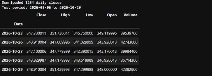
Now download five years of daily Apple stock data. Setting auto_adjust=True returns closing prices adjusted for splits and dividends.
data = yf.download(
    TICKER,
    period="5y",
    interval="1d",
    auto_adjust=True,
    multi_level_index=False,
    progress=False,
)

close = data["Close"].dropna().astype(float)

assert len(close) >= WINDOW + DAYS
assert (close > 0).all()
display(data.tail())
We use the last 60 trading sessions for testing and the preceding 500 observations as context for each prediction.
2. Load Timestral on your GPU
Load the 209M model onto the GPU, with a CPU fallback if CUDA is not available. The 837 MB of weights download from Hugging Face the first time you run this cell.
device = "cuda" if torch.cuda.is_available() else "cpu"

model = TimestralForecaster.from_pretrained(
    MODEL,
    device=device,
)

print(f"Loaded {MODEL} on {device}")
Our model loaded successfully on the RTX 4070:
Loaded mistralai/Timestral-209M on cuda
3. Generate rolling one-day forecasts
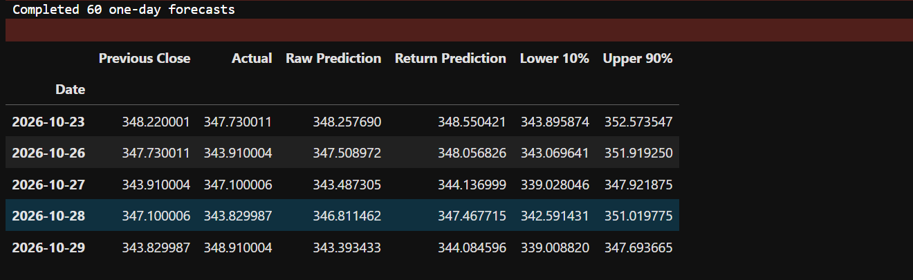
Now we generate two predictions for each trading day: one from historical closing prices and one from log returns. A log return is the day-to-day change in the logarithm of the price, and we convert each predicted return back into a price using the previous close.
actual = []
price_predictions = []
return_predictions = []
previous_prices = []
lower_bounds = []
upper_bounds = []
dates = []
for i in tqdm(range(DAYS), desc="Forecasting"):
pos = len(close) - DAYS + i
history = close.iloc[pos - WINDOW:pos].to_numpy(dtype=np.float32)
previous = float(history[-1])
with torch.inference_mode():
price_fc = model.forecast(
history,
prediction_length=1,
)
price_pred = float(price_fc.median.squeeze())
returns = np.diff(np.log(history))
return_fc = model.forecast(
returns.astype(np.float32),
prediction_length=1,
)
return_pred = previous * np.exp(
float(return_fc.median.squeeze())
)
actual.append(float(close.iloc[pos]))
previous_prices.append(previous)
price_predictions.append(price_pred)
return_predictions.append(return_pred)
lower_bounds.append(float(price_fc.quantile(0.1).squeeze()))
upper_bounds.append(float(price_fc.quantile(0.9).squeeze()))
dates.append(close.index[pos])
actual = np.array(actual)
previous_prices = np.array(previous_prices)
price_predictions = np.array(price_predictions)
return_predictions = np.array(return_predictions)
lower_bounds = np.array(lower_bounds)
upper_bounds = np.array(upper_bounds)
results = pd.DataFrame({
"Previous Close": previous_prices,
"Actual": actual,
"Raw Prediction": price_predictions,
"Return Prediction": return_predictions,
"Lower 10%": lower_bounds,
"Upper 90%": upper_bounds,
}, index=pd.DatetimeIndex(dates, name="Date"))
display(results.tail())
The model generates 60 rolling one-day forecasts, using the previous 500 closing prices for each one. Each forecast uses only data available before the target day, so future prices cannot leak into the model's inputs.
4. Evaluate forecast accuracy
We measure mean absolute error (MAE), root mean squared error (RMSE), mean absolute percentage error (MAPE), and directional accuracy. We also compare Timestral against a naive baseline that assumes tomorrow's closing price will equal today's.
actual = results["Actual"].to_numpy()
previous = results["Previous Close"].to_numpy()
raw = results["Raw Prediction"].to_numpy()
ret = results["Return Prediction"].to_numpy()

def evaluate(prediction, baseline=False):
    metrics = {
        "MAE ($)": np.mean(np.abs(actual - prediction)),
        "RMSE ($)": np.sqrt(np.mean((actual - prediction) ** 2)),
        "MAPE (%)": np.mean(np.abs((actual - prediction) / actual)) * 100,
    }
    metrics["Direction (%)"] = (
        np.nan if baseline
        else np.mean(np.sign(actual - previous) == np.sign(prediction - previous)) * 100
    )
    return metrics

metrics = pd.DataFrame({
    "Baseline": evaluate(previous, baseline=True),
    "Raw Prices": evaluate(raw),
    "Log Returns": evaluate(ret),
}).T

coverage = (
    (actual >= results["Lower 10%"].to_numpy())
    & (actual <= results["Upper 90%"].to_numpy())
).mean() * 100

display(metrics.round(2))
print(f"Raw-price 10-90% interval coverage: {coverage:.1f}%")
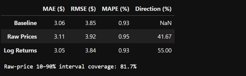
Our results show that Timestral performs slightly better when forecasting log returns instead of raw stock prices.
The log-returns approach achieved the lowest MAE ($3.05), RMSE ($3.84), and MAPE (0.93%), narrowly outperforming our baseline model.
More importantly, directional accuracy improved from 41.67% with raw prices to 55% with log returns, suggesting better performance in predicting whether stock prices will rise or fall.
The raw-price model also achieved 81.7% prediction interval coverage, close to the expected 80%, indicating reasonably calibrated uncertainty estimates. Overall, Timestral generated fairly accurate price forecasts, but its improvement over the simple baseline was minimal, and further testing is needed to determine whether its predictions can reliably support trading decisions.
5. Visualize Timestral predictions
Let's plot the actual closing prices against both forecasting methods using Matplotlib.
fig, axes = plt.subplots(
2, 1,
figsize=(14, 9),
gridspec_kw={"height_ratios": [2, 1]},
sharex=True,
)
axes[0].plot(
dates, actual,
label="Actual Price",
color="green",
linewidth=2.5,
)
axes[0].plot(
dates, price_predictions,
label="Timestral Raw Price",
color="orange",
linestyle="--",
)
axes[0].plot(
dates, return_predictions,
label="Timestral Log Returns",
color="royalblue",
linestyle="--",
)
axes[0].fill_between(
dates,
lower_bounds,
upper_bounds,
color="orange",
alpha=0.12,
label="10-90% Forecast Range",
)
axes[0].set_title(f"Timestral-209M | {TICKER} Rolling One-Day Forecast")
axes[0].set_ylabel("Adjusted Close (USD)")
axes[0].legend()
axes[0].grid(alpha=0.2)
axes[1].plot(
dates,
price_predictions - actual,
label="Raw Price Error",
color="orange",
)
axes[1].plot(
dates,
return_predictions - actual,
label="Log Return Error",
color="royalblue",
)
axes[1].axhline(0, color="black", linestyle=":")
axes[1].set_ylabel("Error ($)")
axes[1].set_xlabel("Date")
axes[1].legend()
axes[1].grid(alpha=0.2)
fig.autofmt_xdate()
plt.tight_layout()
fig.savefig("aapl_improved.png", dpi=180, bbox_inches="tight")
plt.show()
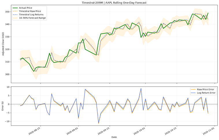
The chart shows how closely Timestral follows Apple's actual prices across the 60 trading days. Both approaches capture the upward trend, and the shaded orange area is the raw-price model's 10-90% prediction interval. The bottom panel plots daily prediction errors.
Most errors stay within about $5, with a few larger misses of $9 to $11 during sudden price moves. The two methods produce nearly identical forecasts, with log returns slightly ahead. Both forecast lines also trail the actual price by roughly one day, which fits with how small the gap to the naive baseline is.
6. Generate Buy, Hold, and Sell signals
Now let's convert the raw-price predictions into experimental Buy, Hold, and Sell signals. We use a 1% threshold on the predicted price change:
- BUY: Predicted price increase greater than 1%.
- SELL: Predicted price decrease greater than 1%.
- HOLD: Predicted price movement between -1% and +1%.
We can implement these rules with NumPy:
THRESHOLD = 1.0

change_pct = (
    price_predictions / previous_prices - 1
) * 100

signals = np.where(
    change_pct > THRESHOLD,
    "BUY",
    np.where(change_pct < -THRESHOLD, "SELL", "HOLD"),
)

results["Expected Change (%)"] = change_pct
results["Signal"] = signals

display(results.tail(10).round(2))
display(results["Signal"].value_counts())

results.to_csv("aapl_signals.csv")
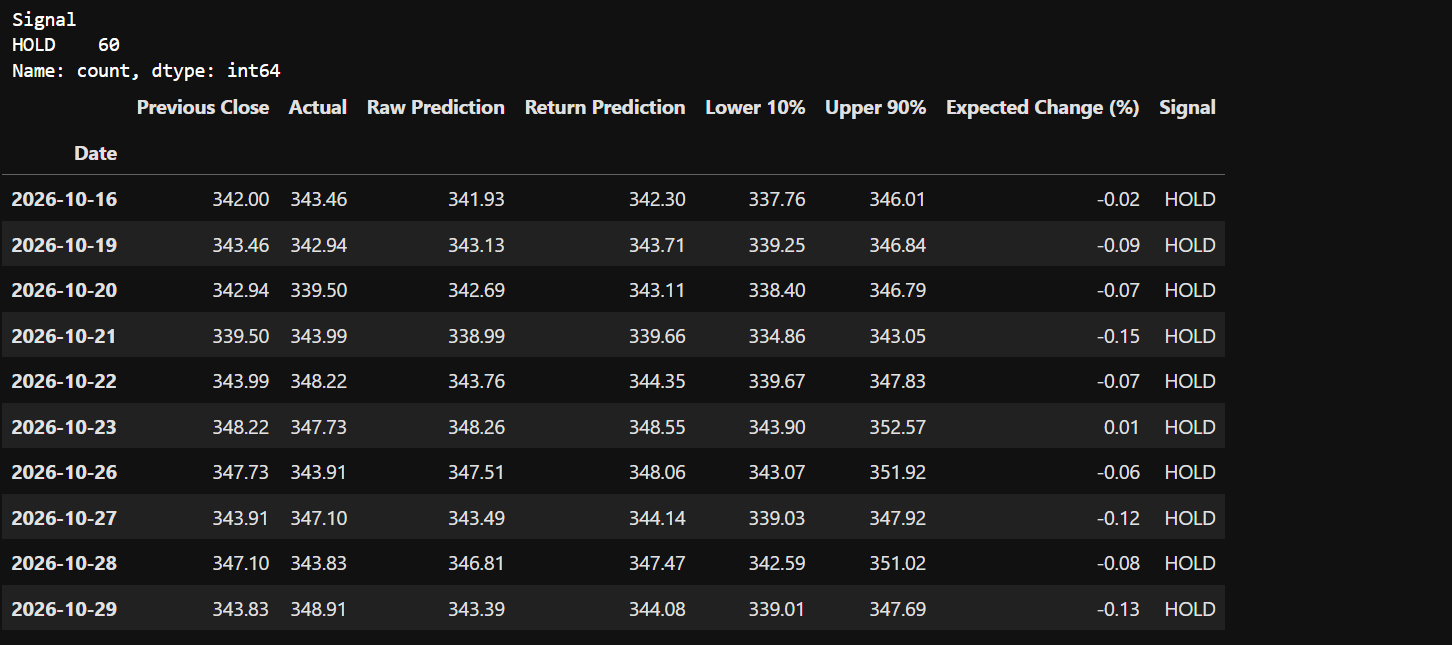
All 60 trading days produced HOLD signals, with no BUY or SELL recommendations. In the last 10 rows shown, the expected change never exceeds 0.15% in either direction, far below our 1% threshold.
These signals come from the raw-price predictions, which had the weaker directional accuracy (41.67%). To see signals from the log-return forecasts instead, swap price_predictions for return_predictions in the change_pct calculation. A lower threshold would produce more BUY and SELL signals, but it would also make them more sensitive to forecasting errors and market noise.
These signals are for experimentation, not live trading, and nothing in this tutorial is financial advice. Further backtesting, threshold tuning, and transaction cost analysis would be necessary to find out whether they could support a profitable strategy.
Final Thoughts
Overall, I am really impressed with Timestral.
The entire setup was straightforward, inference was fast, and I could run everything locally on my RTX 4070 without relying on external APIs.
What makes it even more appealing is that these lightweight models can also run on CPUs, making them accessible without expensive hardware.
When it comes to forecasting accuracy, our results were mixed.
Timestral followed stock prices reasonably well, but it barely outperformed a simple baseline.
I am not an expert in financial forecasting or trading, so there is probably more I could do with data preparation, forecasting strategies, and parameter tuning to get better results.
I have previously used hosted forecasting services such as TimeGPT, but Timestral has made local forecasting much more attractive. Since its release, I have started moving more of my forecasting workloads to local models because they are fast, lightweight, and free of API calls and usage-based fees.
For me, Timestral's biggest strength is not just accuracy, but how easy and inexpensive it makes forecasting.
You can run a capable time-series model on your own hardware, experiment freely, and build it into applications without depending on external services. Even if our stock predictions were not impressive, I think Timestral is an excellent option for anyone building local forecasting applications.
If you're keen to learn more about forecasting, I recommend checking out our Time Series Analysis in Python course. For finance-specific modeling, try Machine Learning for Finance in Python.



What if you could forecast stock prices with a small AI model that runs locally, returns predictions in milliseconds, and needs no additional training?
Time-series forecasting usually means statistical methods such as ARIMA, machine learning pipelines, or models trained on a specific dataset. Timestral, a family of open-weight forecasting models released by Mistral AI on October 15, 2026, takes a different approach. It predicts future values from historical data without fine-tuning, and according to Mistral, its largest model ranks first among pretrained zero-shot models on three public benchmarks.
Despite their small size, the models deliver competitive accuracy across multiple forecasting benchmarks and can be applied to everything from financial markets to energy consumption and retail demand.
In this tutorial, we will look at what Timestral is and how it works, set it up locally with Python and uv, and test it on real Apple (AAPL) stock data. We will generate rolling one-day forecasts, compare them against actual closing prices and a naive baseline, and turn the predictions into simple Buy, Sell, or Hold signals. You can also see our tutorials on time series forecasting with TimeGPT and ARIMA for time series forecasting.
What Is Mistral Timestral?
Timestral is an open-weight time-series foundation model family from Mistral AI for fast, general-purpose forecasting. A time-series foundation model is pretrained once on a large, varied collection of series, so it can forecast data it has never seen.
Unlike traditional forecasting models that need training on a specific dataset, Timestral supports zero-shot forecasting. It predicts future values directly from historical data, with no additional training or fine-tuning.
Timestral is a causal, patch-based transformer trained mostly on synthetic data, followed by a second training stage on a mix of real and synthetic data. It handles stock prices, energy demand, sales, and sensor measurements. Mistral describes the architecture and training in its technical report.
Mistral released four sizes, each with a different trade-off between model size, speed, and accuracy:
According to Mistral's published benchmarks, Timestral-209M ranks first among pretrained and zero-shot models on GIFT-Eval, TIME, and fev-bench. It beats larger models such as TimesFM-3 and Falcon-2.0 in the reported comparisons. These are Mistral's own results, submitted to the GIFT-Eval and TIME leaderboards, so check the leaderboards for independent confirmation.
Speed is another advantage. On a standard server CPU with 8 threads, Mistral reports that Timestral-209M forecasts one day ahead from three weeks of 15-minute history in 113 milliseconds, and the 5M model takes 17 milliseconds. No GPU is required.
Timestral supports these forecasting features:
For this tutorial, we will use Timestral-209M, the largest and most accurate model in the family according to Mistral's published benchmarks. We will run it locally on an NVIDIA RTX 4070 GPU to forecast stock prices and evaluate its performance on real market data.
Set Up Timestral on Linux
Timestral needs Python 3.10 or later and PyTorch 2.4 or later. We will use Python 3.12, PyTorch 2.7.0, and uv to create a lightweight development environment on a Linux machine. Timestral also supports CPU inference, so a GPU is optional.
First, verify that your NVIDIA GPU is detected and its drivers are working:
This command displays your GPU information, driver version, and CUDA compatibility. If your GPU appears in the output, you can proceed.
Next, install uv, a fast Python package and environment manager:
Restart your terminal after installing uv so the command becomes available in your shell.
Now create a project directory and a Python 3.12 virtual environment:
Next, install PyTorch 2.7.0 with CUDA 12.6 support:
During testing, the CUDA 12.8 build threw a driver compatibility error on our RTX 4070. Switching to PyTorch 2.7.0 with CUDA 12.6 fixed it without a driver update. Depending on your GPU and NVIDIA driver, you may need a different CUDA build.
If you do not have a GPU, install the CPU build instead by replacing the index URL with
https://download.pytorch.org/whl/cpu. The code later in this tutorial falls back to the CPU automatically.Now install Timestral directly from its official GitHub repository:
Install the remaining libraries for downloading stock market data, processing predictions, creating visualizations, and running notebooks:
We use yfinance to retrieve historical stock prices, pandas and NumPy for data processing, and Matplotlib for plotting actual versus predicted prices. We also constrain the pandas version to the range used during our testing to avoid compatibility-related warnings.
Before proceeding, verify that PyTorch can access your GPU:
Our output:
The
Truevalue confirms that CUDA is available to PyTorch, and the final line identifies the GPU. We are now ready to start experimenting with Timestral.Instead of separate Python scripts, we will use JupyterLab so we can run code step by step, inspect forecast values, and compare predictions against actual market data. Launch JupyterLab from your project directory:
Open the URL displayed in your terminal, usually
http://localhost:8888/lab, and create a new Python notebook using the environment we just configured. We will use this notebook to load Timestral, generate predictions, and evaluate how well the model performs.Forecast Apple Stock Prices With Timestral
Rather than generating synthetic data, we will use real historical Apple stock prices and measure how accurately Timestral predicts the next trading day's closing price.
To make the experiment more realistic, we will use rolling one-day forecasting. For every trading day in the test period, Timestral receives the previous 500 closing prices and predicts only the following day's close.
We will also compare two methods:
1. Download historical stock prices
Start a notebook and import the required libraries. We also set the ticker, the number of test days, the context window, and the model name.
Now download five years of daily Apple stock data. Setting
auto_adjust=Truereturns closing prices adjusted for splits and dividends.We use the last 60 trading sessions for testing and the preceding 500 observations as context for each prediction.
2. Load Timestral on your GPU
Load the 209M model onto the GPU, with a CPU fallback if CUDA is not available. The 837 MB of weights download from Hugging Face the first time you run this cell.
Our model loaded successfully on the RTX 4070:
3. Generate rolling one-day forecasts
Now we generate two predictions for each trading day: one from historical closing prices and one from log returns. A log return is the day-to-day change in the logarithm of the price, and we convert each predicted return back into a price using the previous close.
The model generates 60 rolling one-day forecasts, using the previous 500 closing prices for each one. Each forecast uses only data available before the target day, so future prices cannot leak into the model's inputs.
4. Evaluate forecast accuracy
We measure mean absolute error (MAE), root mean squared error (RMSE), mean absolute percentage error (MAPE), and directional accuracy. We also compare Timestral against a naive baseline that assumes tomorrow's closing price will equal today's.
Our results show that Timestral performs slightly better when forecasting log returns instead of raw stock prices.
The log-returns approach achieved the lowest MAE ($3.05), RMSE ($3.84), and MAPE (0.93%), narrowly outperforming our baseline model.
More importantly, directional accuracy improved from 41.67% with raw prices to 55% with log returns, suggesting better performance in predicting whether stock prices will rise or fall.
The raw-price model also achieved 81.7% prediction interval coverage, close to the expected 80%, indicating reasonably calibrated uncertainty estimates. Overall, Timestral generated fairly accurate price forecasts, but its improvement over the simple baseline was minimal, and further testing is needed to determine whether its predictions can reliably support trading decisions.
5. Visualize Timestral predictions
Let's plot the actual closing prices against both forecasting methods using Matplotlib.
The chart shows how closely Timestral follows Apple's actual prices across the 60 trading days. Both approaches capture the upward trend, and the shaded orange area is the raw-price model's 10-90% prediction interval. The bottom panel plots daily prediction errors.
Most errors stay within about $5, with a few larger misses of $9 to $11 during sudden price moves. The two methods produce nearly identical forecasts, with log returns slightly ahead. Both forecast lines also trail the actual price by roughly one day, which fits with how small the gap to the naive baseline is.
6. Generate Buy, Hold, and Sell signals
Now let's convert the raw-price predictions into experimental Buy, Hold, and Sell signals. We use a 1% threshold on the predicted price change:
We can implement these rules with NumPy:
All 60 trading days produced HOLD signals, with no BUY or SELL recommendations. In the last 10 rows shown, the expected change never exceeds 0.15% in either direction, far below our 1% threshold.
These signals come from the raw-price predictions, which had the weaker directional accuracy (41.67%). To see signals from the log-return forecasts instead, swap
price_predictionsforreturn_predictionsin thechange_pctcalculation. A lower threshold would produce more BUY and SELL signals, but it would also make them more sensitive to forecasting errors and market noise.These signals are for experimentation, not live trading, and nothing in this tutorial is financial advice. Further backtesting, threshold tuning, and transaction cost analysis would be necessary to find out whether they could support a profitable strategy.
Final Thoughts
Overall, I am really impressed with Timestral.
The entire setup was straightforward, inference was fast, and I could run everything locally on my RTX 4070 without relying on external APIs.
What makes it even more appealing is that these lightweight models can also run on CPUs, making them accessible without expensive hardware.
When it comes to forecasting accuracy, our results were mixed.
Timestral followed stock prices reasonably well, but it barely outperformed a simple baseline.
I am not an expert in financial forecasting or trading, so there is probably more I could do with data preparation, forecasting strategies, and parameter tuning to get better results.
I have previously used hosted forecasting services such as TimeGPT, but Timestral has made local forecasting much more attractive. Since its release, I have started moving more of my forecasting workloads to local models because they are fast, lightweight, and free of API calls and usage-based fees.
For me, Timestral's biggest strength is not just accuracy, but how easy and inexpensive it makes forecasting.
You can run a capable time-series model on your own hardware, experiment freely, and build it into applications without depending on external services. Even if our stock predictions were not impressive, I think Timestral is an excellent option for anyone building local forecasting applications.
If you're keen to learn more about forecasting, I recommend checking out our Time Series Analysis in Python course. For finance-specific modeling, try Machine Learning for Finance in Python.