ARIMA for Time Series Forecasting: A Complete Guide

Let’s take a look at ARIMA, which is one of the most popular (if not the most popular) time series forecasting techniques. ARIMA is popular because it effectively models time series data by capturing both the autoregressive (AR) and moving average (MA) components, while also addressing non-stationarity through differencing (I). This combination makes ARIMA models especially flexible, which is why they are used across very different industries, like finance and weather prediction. 

ARIMA models are highly technical, but I will break down the parts so you can develop a strong understanding. Before getting started, it's a good idea to familiarize yourself with some foundational tools. DataCamp offers a lot of good resources, such as our ARIMA Models in Python or ARIMA Models in R courses. You can choose either depending on the language you prefer. 

Why Use ARIMA Forecasting? 

Throughout finance, economics and environmental sciences etc., ARIMA has great interest because it can identify many complex patterns of our past observations with future needs which makes it a state-of-the-art technique. From predicting the price of stocks, forecasting weather patterns to getting an idea about consumer demand, ARIMA is a great way to make accurate and actionable predictive analyses.

By using ARIMA, we are able to both analyze and forecast time series data in a sophisticated manner that accounts for patterns, trends, and seasonality. This facilitates a 360-degree view of the underlying dynamics for making informed decisions.

Key Components of ARIMA Models

In order to really understand ARIMA, we need to deconstruct its building blocks. Once we have the components down, it will become easier to understand how this time series forecasting method works as a whole. Here, I’ll give a detailed explanation of every component.

Autoregressive (AR) part

The Autoregressive (AR) component builds a trend from past values in the AR framework for predictive models. For clarification, the 'autoregression framework' works like a regression model where you use the lags of the time series' own past values as the regressors.

Integrated (I) part

The Integrated (I) part involves the differencing of the time series component keeping in mind that our time series should be stationary, which really means that the mean and variance should remain constant over a period of time. Basically, we subtract one observation from another so that trends and seasonality are eliminated. By performing differencing we get stationarity. This step is necessary because it helps the model fit the data and not the noise.

Moving average (MA) part 

The moving average (MA) component focuses on the relationship between an observation and a residual error. Looking at how the present observation is related to those of the past errors, we can then infer some helpful information about any possible trend in our data.

We can consider the residuals among one of these errors, and the moving average model concept estimates or considers their impact on our latest observation. This is particularly useful for tracking and trapping short-term changes in the data or random shocks. In the (MA) part of a time series, we can gain valuable information about its behavior which in turn allows us to forecast and predict with greater accuracy.

How to Build an ARIMA Model in Python

To build an ARIMA model for forecasting, like gold prices, you can follow these steps. Let’s break it down together.

Data collection 

The first step is to tee up an appropriate dataset and prepare our environment.

Find a dataset

Collect or search for a dataset from data source platforms. You want one that has historical data over time. Here is a link to the Kaggle dataset related to gold future prices. 

Install packages

We install the packages we need, including statsmodels and sklearn. 

import pandas as pd
import matplotlib.pyplot as plt
from statsmodels.tsa.stattools import adfuller
from statsmodels.graphics.tsaplots import plot_acf, plot_pacf
from statsmodels.tsa.arima.model import ARIMA
from sklearn.metrics import mean_squared_error

Load the data

We then read the data into our local environment. I'm taking the extra step to make sure the dates are recognized in order.

# Define the path to your CSV file
# You may have to make this path more specific to the location of your file.
csv_path = "future-gc00-daily-prices.csv"

# Read the CSV, parse 'Date' column as datetime, and set it as the index
data = pd.read_csv(
    csv_path,
    parse_dates=["Date"],
    dayfirst=False,
    index_col="Date"
)

# Sort the DataFrame by the Date index in ascending order
data.sort_index(inplace=True)

Data preprocessing 

Our dataset is pretty clean, but in other contexts, we would have to handle indexing issues, which is important in time series forecasting. For example, since we are forecasting the closing value of a stock on a particular exchange, we have to consider that the stock market is not open on weekends.

Before continuing, I'm also taking the quick step of removing commas from the Close variable, which is what I will be using.

# Clean the "Close" column
data["Close"] = data["Close"].replace(',', '', regex=True)
data["Close"] = pd.to_numeric(data["Close"], errors='coerce')
data["Close"].replace([np.inf, -np.inf], np.nan, inplace=True)
data.dropna(subset=["Close"], inplace=True)

Handle missing values

As part of data preprocessing, we also often have to consider how to handle missing values using an imputation method like forward filling or mean replacement. Do know that even one NA value, depending on the programming language and the library you are using, can prevent an ARIMA from running.

I had mentioned that weekend days might be recognized as NA. That's can be the case, and would require an extra step. Luckily, statsmodels treats the data as a sequential index without strictly enforcing regular time intervals, allowing our model to compile even weekend gaps. 

Create a time plot

Now is a good time to create a time plot so we can see the series that we are working with: 

# Plotting the original Close price
plt.figure(figsize=(14, 7))
plt.plot(data.index, data["Close"], label='Close Price')
plt.title('Close Price Over Time')
plt.xlabel('Date')
plt.ylabel('Close Price')
plt.legend()
plt.show()

Check for stationarity and perform differencing if necessary

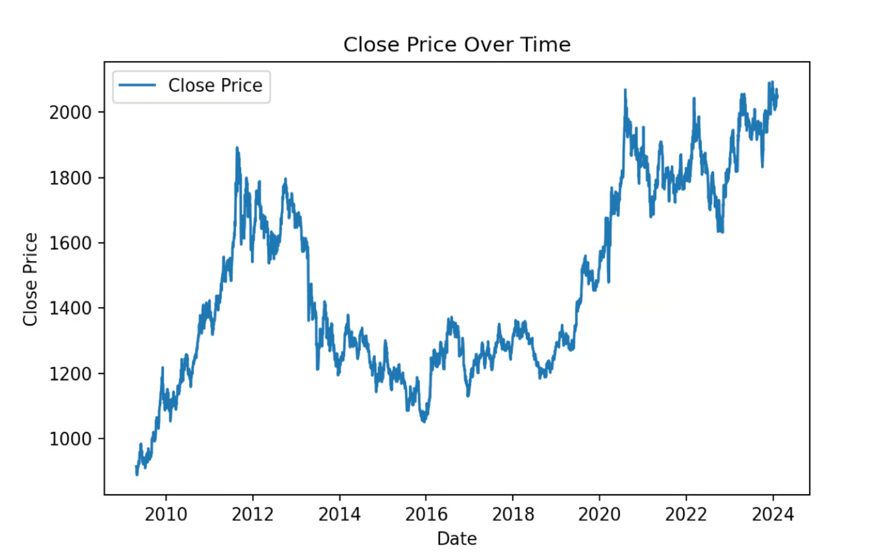
While ARIMA models can deal with non-stationarity up to a point, they cannot effectively account for time-varying variance. In other words, for an ARIMA model to really work, the data has to be stationary.

Looking at the plot, above, we can see that the data is, in fact, not stationary because there is a clear trend. Also, it looks like there is non-constant variance at different time points. We can use the Augmented Dickey-Fuller test to test our intuition and see if our data has a constant mean and variance, and put numbers to it. 

# Perform the Augmented Dickey-Fuller test on the original series
result_original = adfuller(data["Close"])

print(f"ADF Statistic (Original): {result_original[0]:.4f}")
print(f"p-value (Original): {result_original[1]:.4f}")

if result_original[1] < 0.05:
    print("Interpretation: The original series is Stationary.\n")
else:
    print("Interpretation: The original series is Non-Stationary.\n")

# Apply first-order differencing
data['Close_Diff'] = data['Close'].diff()

# Perform the Augmented Dickey-Fuller test on the differenced series
result_diff = adfuller(data["Close_Diff"].dropna())
print(f"ADF Statistic (Differenced): {result_diff[0]:.4f}")
print(f"p-value (Differenced): {result_diff[1]:.4f}")
if result_diff[1] < 0.05:
    print("Interpretation: The differenced series is Stationary.")
else:
    print("Interpretation: The differenced series is Non-Stationary.")

ADF Statistic (Original): -1.4367
p-value (Original): 0.5646
Interpretation: The original series is Non-Stationary.

ADF Statistic (Differenced): -19.1308
p-value (Differenced): 0.0000
Interpretation: The differenced series is Stationary.

The results of our Augmented Dickey-Fuller test indicate that our original series is, in fact, non-stationary, so using an ARIMA out-of-the-box on the original data would be a mistake.

The ADF test on a differenced version of the data indicates that the differenced version is stationary, however.

A quick note on differencing. I want to take the time to explain this, since a lot is happening under the hood. To perform differencing, we subtract each observation from the previous one to give us a new time series of first differences. (The new time series is now one element shorter than the original.) If the differenced series is still not stationary, we can take a second difference by differencing the original series again, and we can continue differencing the series until it finally becomes stationary. The order of differencing required is the minimum number of differences needed to get a series with no autocorrelation.

I do want to say, finally - don't perform differencing more than you have to, otherwise you might create some false dynamics in your data. Also, if you were going to do seasonal ARIMA model, which we aren't doing in this tutorial, you would always consider a seasonal difference before a first difference.

# Plotting the differenced Close price
plt.figure(figsize=(14, 7))
plt.plot(data.index, data['Close_Diff'], label='Differenced Close Price', color='orange')
plt.title('Differenced Close Price Over Time')
plt.xlabel('Date')
plt.ylabel('Differenced Close Price')
plt.legend()
plt.show()

Model identification

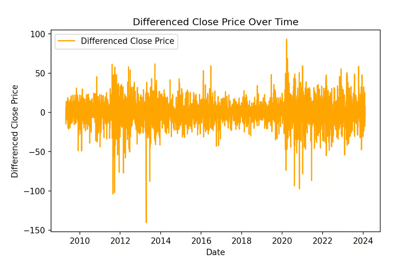
When we build an ARIMA model, we have to consider the p, d, and q terms that go into our ARIMA model. 

• The first parameter, p, is the number of lagged observations. By considering p, we effectively determine how far back in time we go when trying to predict the current observation. We do this by looking at the autocorrelations of our time series, which are the correlations in our series at previous time lags. 
• The second parameter, d, refers to the order of differencing, which we talked about. Again, differencing simply means finding the differences between consecutive timesteps. It is a way to make our data stationary, which means removing the trends and any changes in variance over time. d indicates differencing at which order you get a process stationary.
• The third parameter q refers to the order of the moving average (MA) part of the model. It represents the number of lagged forecast errors included in the model. Unlike a simple moving average, which smooths data, the moving average in ARIMA captures the relationship between an observation and the residual errors from a moving average model applied to lagged observations.

Finding the ARIMA terms

We use tools like ACF (Autocorrelation Function) and PACF (Partial Autocorrelation Function) to determine the values of p, d, and q. The number of lags where ACF cuts off is q, and where PACF cuts off is p. We also have to choose the appropriate value for d by creating a situation where, after differencing, the data resembles white noise. For our data, we choose 1 for both p and q because we see a significant spike in the first lag for each.

from statsmodels.graphics.tsaplots import plot_acf, plot_pacf
import matplotlib.pyplot as plt

# Plot ACF and PACF for the differenced series
fig, axes = plt.subplots(1, 2, figsize=(16, 4))

# ACF plot
plot_acf(data['Close_Diff'].dropna(), lags=40, ax=axes[0])
axes[0].set_title('Autocorrelation Function (ACF)')

# PACF plot
plot_pacf(data['Close_Diff'].dropna(), lags=40, ax=axes[1])
axes[1].set_title('Partial Autocorrelation Function (PACF)')

plt.tight_layout()
plt.show()

Parameter estimation 

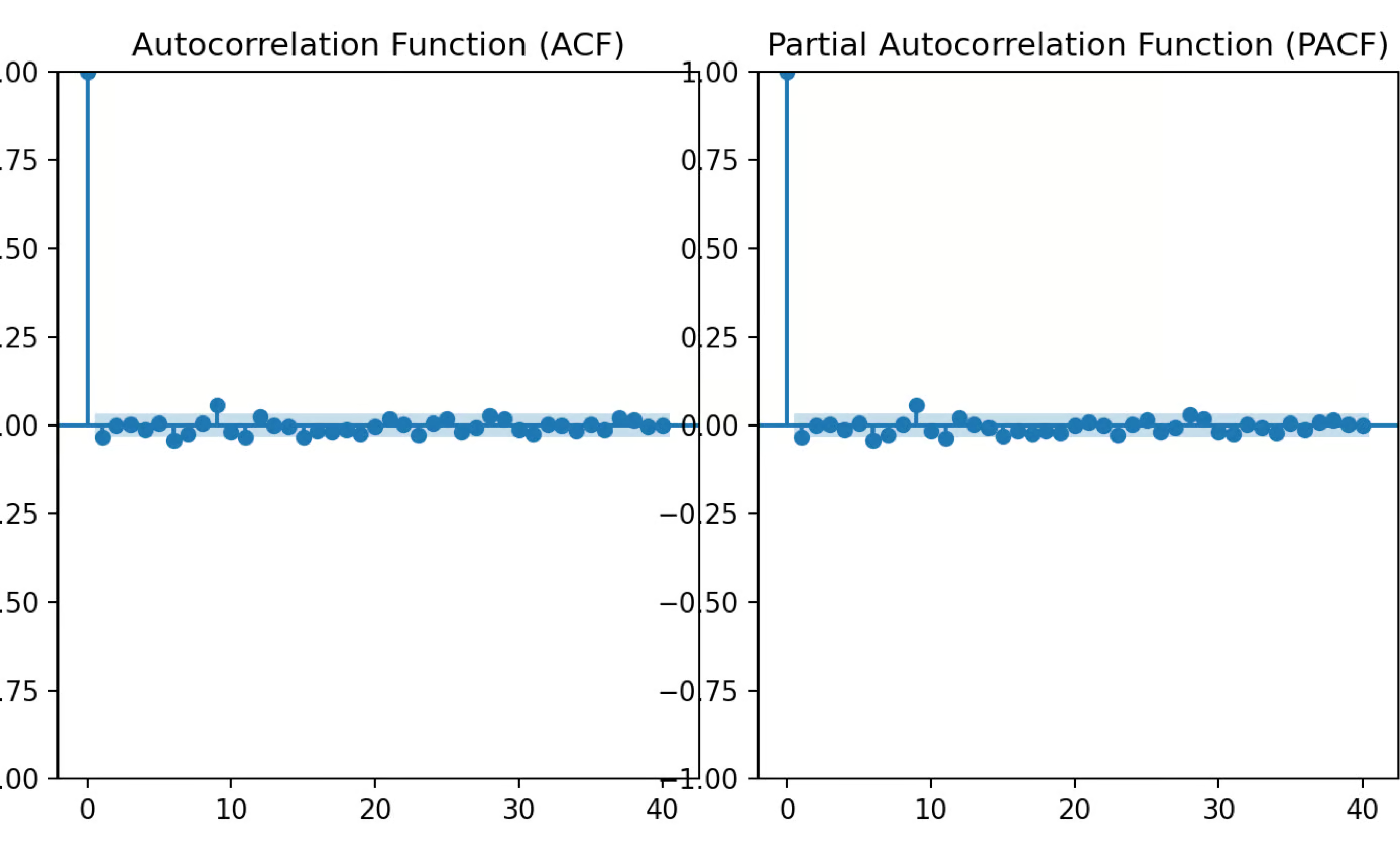
To be clear, the p, d, and q values in ARIMA represent the model's order (lags for autoregression, differencing, and moving average terms), but they are not the actual parameters being estimated. Once the p, d, and q values are chosen, the model estimates additional parameters, such as coefficients for the autoregressive and moving average terms, through maximum likelihood estimation (MLE).

Forecasting

To forecast using an ARIMA model, start by using the fitted model to predict future values based on the data. Once predictions are made, it's helpful to visualize them by plotting the predicted values alongside the actual values. This is accomplished because we use a train/test workflow, where the data is split into training and testing sets. Doing this lets us see how well the model performs on unseen data. If you are unclear on this, take our Model Validation in Python course, which is a great resource to learn the ins and outs of training and testing.

1. Use a train/test workflow

Our first step is to split the data into training and testing versions. 

# Split data into train and test
train_size = int(len(data) * 0.8)
train, test = data.iloc[:train_size], data.iloc[train_size:]

# Fit ARIMA model
model = ARIMA(train["Close"], order=(1,1,1))
model_fit = model.fit()

2. Visualize our time series

Our next step is to create our forecast and also to visually inspect it. We can see how our forecast performs against the testing version of our data.

# Forecast
forecast = model_fit.forecast(steps=len(test))

# Plot the results with specified colors
plt.figure(figsize=(14,7))
plt.plot(train.index, train["Close"], label='Train', color='#203147')
plt.plot(test.index, test["Close"], label='Test', color='#01ef63')
plt.plot(test.index, forecast, label='Forecast', color='orange')
plt.title('Close Price Forecast')
plt.xlabel('Date')
plt.ylabel('Close Price')
plt.legend()
plt.show()

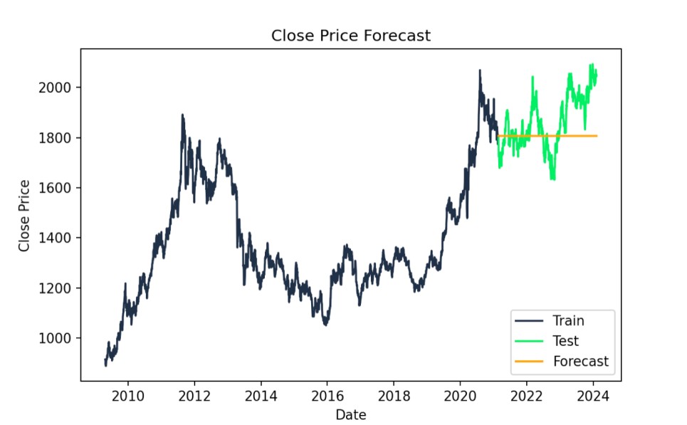
ARIMA forecast actual vs. predicted values. Image by Author

3. Evaluate model statistics

We check out the AIC and BIC model statistics. Lower values mean the model fits better, but we might also compare the results with those from simpler models to avoid overfitting. I'm printing the numbers here but they make the most sense in the context of comparing to other ARIMA models on the same data, in order to find the ARIMA model that works best.

print(f"AIC: {model_fit.aic}")
print(f"BIC: {model_fit.bic}")

AIC: 24602.97426066606
BIC: 24620.97128230579

We can also evaluate the mean squared error, to assess our model's fit. This is a practical metric. A lower RMSE indicates a better ARIMA model, reflecting smaller differences between actual and predicted values, and it's on the scale of the data. That is, the RMSE of 118.5339 signifies that, on average, our model's predictions deviate from the actual Close prices by about $118.53.

forecast = forecast[:len(test)]
test_close = test["Close"][:len(forecast)]

# Calculate RMSE
rmse = np.sqrt(mean_squared_error(test_close, forecast))
print(f"RMSE: {rmse:.4f}")

RMSE: 118.5339