What is A Confusion Matrix in Machine Learning? The Model Evaluation Tool Explained

This year has been one of innovation in the field of data science, with artificial intelligence and machine learning dominating headlines. While there’s no doubt about the progress made in 2023, it’s important to recognize that many of these machine learning advancements have only been possible due to the correct evaluation processes the models undergo. Data practitioners are tasked with ensuring accurate evaluations and processes are taken to measure the performance of a machine learning model. This is not beneficial - it is essential.

If you are looking to grasp the art of data science, this article will guide you through the crucial steps of model evaluation using the confusion matrix, a relatively simple but powerful tool that’s widely used in model evaluation.

So let’s dive in and learn more about the confusion matrix.

What is the Confusion Matrix?

The confusion matrix is a tool used to evaluate the performance of a model and is visually represented as a table. It provides a deeper layer of insight to data practitioners on the model's performance, errors, and weaknesses. This allows for data practitioners to further analyze their model through fine-tuning.

The Confusion Matrix Structure

Let’s learn about the basic structure of a confusion matrix, using the example of identifying an email as spam or not spam.

• True Positive (TP) - Your model predicted the positive class. For example, identifying a spam email as spam.
• True Negative (TN) - Your model correctly predicted the negative class. For example, identifying a regular email as not spam.
• False Positive (FP) - Your model incorrectly predicted the positive class. For example, identifying a regular email as spam.
• False Negative (FN) - Your model incorrectly predicted the negative class. For example, identifying a spam email as a regular email.

To truly grasp the concept of a confusion matrix, have a look at the visualization below:

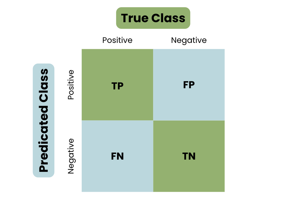
The Basic Structure of a Confusion Matrix

Confusion Matrix Terminology

To have an in-depth understanding of the Confusion Matrix, it is essential to understand the important metrics used to measure the performance of a model.

Let’s define important metrics:

Accuracy

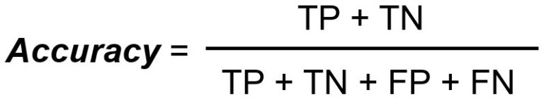
Accuracy measures the total number of correct classifications divided by the total number of cases.

Recall/Sensitivity

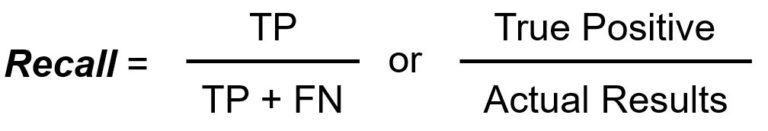
Recall/Sensitivity measures the total number of true positives divided by the total number of actual positives.

Precision

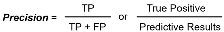
Precision measures the total number of true positives divided by the total number of predicted positives.

Specificity

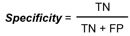
Specificity measures the total number of true negatives divided by the total number of actual negatives.

F1 Score

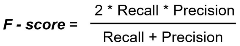
F1 Score is a single metric that is a harmonic mean of precision and recall.

The Role of a Confusion Matrix

To better comprehend the confusion matrix, you must understand the aim and why it is widely used.

When it comes to measuring a model’s performance or anything in general, people focus on accuracy. However, being heavily reliant on the accuracy metric can lead to incorrect decisions. To understand this, we will go through the limitations of using accuracy as a standalone metric.

Limitations of accuracy as a standalone metric

As defined above, accuracy measures the total number of correct classifications divided by the total number of cases. However, using this metric as a standalone comes with limitations, such as:

• Working with Imbalanced Data: No data ever comes perfect, and the use of the accuracy metric should be evaluated on its predictive power. For example, working with a dataset where one class outweighs another will cause the model to achieve a higher accuracy rate as it will predict the majority class.
• Error Types: Understanding and learning about your model's performance in a specific context will aid you in fine-tuning and improving its performance. For example, differentiating between the types of errors through a confusion matrix, such as FP and FN, will allow you to explore the model's limitations.

Through these limitations, the confusion matrix, along with the variety of metrics, offers more detailed insight on how to improve a model’s performance.

The benefits of a confusion matrix

As seen in the basic structure of a confusion matrix, the predictions are broken down into four categories: True Positive, True Negative, False Positive, and False Negative.

This detailed breakdown offers valuable insight and solutions to improve a model's performance:

• Solving Imbalanced Data: As explored, using accuracy as a standalone metric has limitations when it comes to imbalanced data. Using other metrics, such as precision and recall, allows a more balanced view and accurate representation. For example, false positives and false negatives can lead to high consequences in sectors such as Finance.
• Error Type Differentiator: Understanding the different types of errors produced by the machine learning model provides knowledge of its limitations and areas of improvement.
• Trade-Offs: The trade-off between using different metrics in a Confusion Matrix is essential as they impact one another. For example, an increase in precision typically leads to a decrease in recall. This will guide you in improving the performance of the model using knowledge from impacted metric values.

Calculating a Confusion Matrix

Now that we have a good understanding of a basic confusion matrix, its terminology, and its use, let’s move on to manually calculating a confusion matrix, followed by a practical example.

Manually calculating a confusion matrix

Here is a step-by-step guide on how to manually calculate a Confusion Matrix.

Define the outcomes

The first step will be to identify the two possible outcomes of your task: Positive or Negative.

Collecting the predictions

Once your possible outcomes are defined, the next step will be to collect all the model’s predictions, including how many times the model predicted each class and its occurrence.

Classifying the outcomes

Once all the predictions have been collated, the next step is to classify the outcomes into the four categories:

• True Positive (TP)
• True Negative (TN)
• False Positive (FP)
• False Negative (FN)

Create a matrix

Once the outcomes have been classified, the next step is to present them in a matrix table, to be further analyzed using a variety of metrics.

Confusion matrix practical example

Let’s go through a practical example to demonstrate this process.

Continuing to use the same example of identifying an email as spam or not spam, let’s create a hypothetical dataset where spam is Positive and not spam is Negative. We have the following data:

• Amongst the 200 emails, 80 emails are actually spam in which the model correctly identifies 60 of them as spam (TP).
• Amongst the 200 emails, 120 emails are not spam in which the model correctly identifies 100 of them as not spam (TN).
• Amongst the 200 emails, the model incorrectly identifies 20 non-spam emails as spam (FP).
• Amongst the 200 emails, the model misses 20 spam emails and identifies them as non-spam (FN).

At this point, we have defined the outcome and collected the data; the next step is to classify the outcomes into the four categories:

• True Positive: 60
• True Negative: 100
• False Positive: 20
• False Negative: 20

The next step is to turn this into a Confusion Matrix:

So what does the Confusion Matrix tell us?

• The True Positives and True Negatives indicate accurate predictions.
• The False Positives indicate the model incorrectly predicted the positive class.
• The False Negatives indicate the model failed to identify and predict the positive class.

Using this confusion matrix, we can calculate the different metrics: Accuracy, Recall/Sensitivity, Precision, Specificity, and the F1 Score.

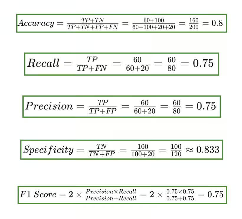
Confusion matrix metrics output

Precision vs. Recall

You may be wondering why the F1 score includes precision and recall in its formula. The F1 score metric is crucial when dealing with imbalanced data or when you want to balance the trade-off between precision and recall.

Precision measures the accuracy of positive prediction. It answers the question of ‘when the model predicted TRUE, how often was it right?’. Precision, in particular, is important when the cost of a false positive is high.

Recall or sensitivity measures the number of actual positives correctly identified by the model. It answers the question of ‘When the class was actually TRUE, how often did the classifier get it right?’.

Recall is important when missing a positive instance (FN) is shown to be significantly worse than incorrectly labeling negative instances as positive.

• Precision use: False positives can have serious consequences. For example, a classification model used in the finance sector wrongfully identified a transaction as fraudulent. In scenarios such as this, the precision metric is important.
• Recall use: Identifying all positive cases can be imperative. For example, classification models used in the medical field failing to diagnose correctly can be detrimental. In scenarios in which correctly identifying all positive cases is essential, the recall metric is important.

Confusion Matrix Using Scikit-learn in Python

To put this into perspective, let’s create a confusion matrix using Scikit-learn in Python, using a Random Forest classifier.

The first step will be to import the required libraries and build your synthetic dataset.

# Import Libraries
from sklearn.datasets import make_classification
from sklearn.model_selection import train_test_split
from sklearn.ensemble import RandomForestClassifier
from sklearn.metrics import confusion_matrix
import matplotlib.pyplot as plt
import seaborn as sns

# Synthetic Dataset
X, y = make_classification(n_samples=1000, n_features=20,
                           n_classes=2, random_state=42)

# Split into Training and Test Sets
X_train, X_test, y_train, y_test = train_test_split(X, y, test_size=0.3, random_state=42)

The next step is to train the model using a simple random forest classifier

# Train the Model
model = RandomForestClassifier(random_state=42)
model.fit(X_train, y_train)

As we did with the practical example, we will need to classify the outcomes and turn it into a confusion matrix. We do this by predicting on the test data first and then generating a Confusion Matrix:

# Predict on the Test Data
y_pred = model.predict(X_test)

# Generate the confusion matrix
cm = confusion_matrix(y_test, y_pred)

Now we want to generate a visual representation of the confusion matrix:

# Create a Confusion Matrix
plt.figure(figsize=(8, 8))
sns.heatmap(cm, annot=True, fmt='d', cmap='Greens')
plt.title('Confusion Matrix')
plt.ylabel('True label')
plt.xlabel('Predicted label')
plt.show()

This is the output:

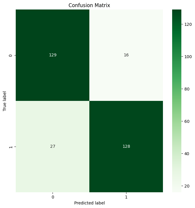
Random Forest Confusion Matrix Output

Tada 🎉 You have successfully created your first Confusion Matrix using Scikit-learn!

Conclusion

In this article, we have explored the definition of a Confusion Matrix, important terminology surrounding the evaluation tool, and the limitations and importance of the different metrics. Being able to manually calculate a Confusion Matrix is important to your data science knowledge base, as well as being able to execute it using libraries such as Scikit-learn.

If you would like to dive further into Confusion Matrix, practice confusion matrices in R with Understanding Confusion Matrix in R. Dive a little deeper with our Model Validation in Python course, where you will learn the basics of model validation, validation techniques and begin creating validated and high performing models.