Random Forest Classification with Scikit-Learn

How Random Forest Classification Works

Imagine you have a complex problem to solve, and you gather a group of experts from different fields to provide their input. Each expert provides their opinion based on their expertise and experience. Then, the experts would vote to arrive at a final decision.

In a random forest classification, multiple decision trees are created using different random subsets of the data and features. Each decision tree is like an expert, providing its opinion on how to classify the data. Predictions are made by calculating the prediction for each decision tree and then taking the most popular result. (For regression, predictions use an averaging technique instead.)

In the diagram below, we have a random forest with n decision trees, and we’ve shown the first 5, along with their predictions (either “Dog” or “Cat”). Each tree is exposed to a different number of features and a different sample of the original dataset, and as such, every tree can be different. Each tree makes a prediction.

Looking at the first 5 trees, we can see that 4/5 predicted the sample was a Cat. The green circles indicate a hypothetical path the tree took to reach its decision. The random forest would count the number of predictions from decision trees for Cat and for Dog, and choose the most popular prediction.

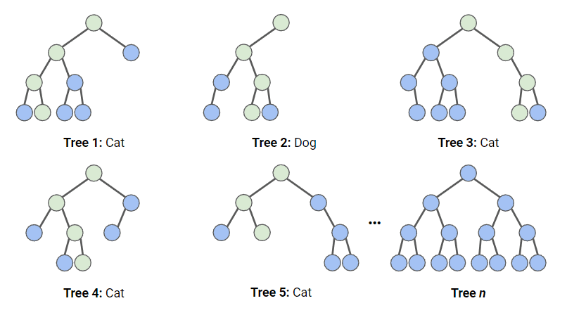Illustration of how random forest classification works. Image by Author

Load the Dataset

This dataset consists of direct marketing campaigns by a Portuguese banking institution using phone calls. The campaigns aimed to sell subscriptions to a bank term deposit. We are going to store this dataset in a variable called bank_data. The columns we will use are:

• age: The age of the person who received the phone call
• default: Whether the person has credit in default
• cons.price.idx: Consumer price index score at the time of the call
• cons.conf.idx:Consumer confidence index score at the time of the call
• y: Whether the person subscribed (this is what we’re trying to predict)

Importing Packages

The following packages and functions are used in this tutorial:

# Data Processing
import pandas as pd
import numpy as np

# Modelling
from sklearn.ensemble import RandomForestClassifier
from sklearn.metrics import accuracy_score, confusion_matrix, precision_score, recall_score, ConfusionMatrixDisplay
from sklearn.model_selection import RandomizedSearchCV, train_test_split
from scipy.stats import randint

# Tree Visualisation
from sklearn.tree import export_graphviz
from IPython.display import Image
import graphviz

The Random Forest Workflow

To fit and train this model, we’ll be following The Machine Learning Workflow infographic; however, as our data is pretty clean, we won’t be carrying out every step. We will do the following:

• Feature engineering
• Split the data
• Train the model
• Hyperparameter tuning
• Assess model performance

Preprocessing Data for our Random Forest Classifier

Tree-based models are much more robust to outliers than linear models, and they do not need variables to be normalized to work. As such, we need to do very little preprocessing on our data.

• We will map our default column, which contains no and yes, to 0s and 1s, respectively. We will treat unknown values as no for this example.
• We will also map our target, y, to 1s and 0s.

bank_data['default'] = bank_data['default'].map({'no':0,'yes':1,'unknown':0})
bank_data['y'] = bank_data['y'].map({'no':0,'yes':1})

Splitting the Data

When training any supervised learning model, it is important to split the data into training and test data. The training data is used to fit the model. The algorithm uses the training data to learn the relationship between the features and the target. The test data is used to evaluate the performance of the model.

The code below splits the data into separate variables for the features and target, then splits into training and test data.

# Split the data into features (X) and target (y)
X = bank_data.drop('y', axis=1)
y = bank_data['y']

# Split the data into training and test sets
X_train, X_test, y_train, y_test = train_test_split(X, y, test_size=0.2)

Fitting and Evaluating the Random Forest Model

We first create an instance of the Random forest model with the default parameters. We then fit this to our training data. We pass both the features and the target variable so the model can learn.

rf = RandomForestClassifier()
rf.fit(X_train, y_train)

At this point, we have a trained random forest model, but we need to find out whether it makes accurate predictions.

y_pred = rf.predict(X_test)

The simplest way to evaluate this model is using accuracy; we check the predictions against the actual values in the test set and count up how many the model got right.

accuracy = accuracy_score(y_test, y_pred)
print("Accuracy:", accuracy)

Output:

Accuracy: 0.888

This is a pretty good score! However, we may be able to do better by optimizing our hyperparameters. 

Visualizing the Results

We can use the following code to visualize our first 3 trees.

# Export the first three decision trees from the forest

for i in range(3):
    tree = rf.estimators_[i]
    dot_data = export_graphviz(tree,
                               feature_names=X_train.columns,  
                               filled=True,  
                               max_depth=2, 
                               impurity=False, 
                               proportion=True)
    graph = graphviz.Source(dot_data)
    display(graph)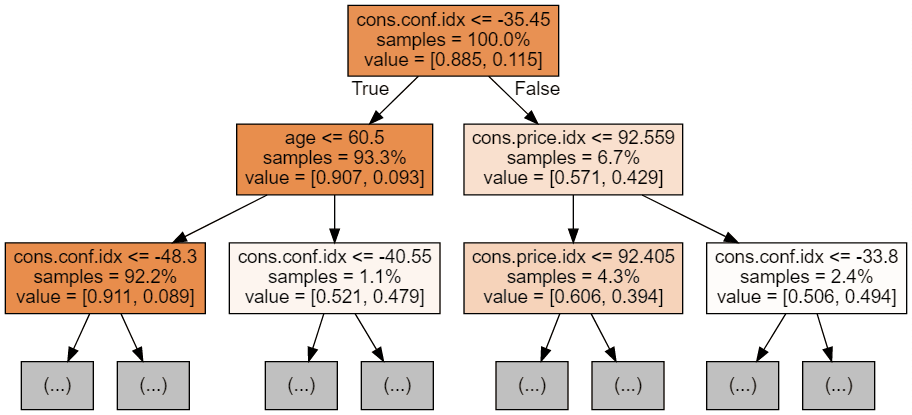

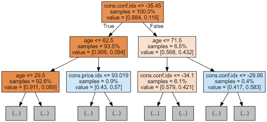
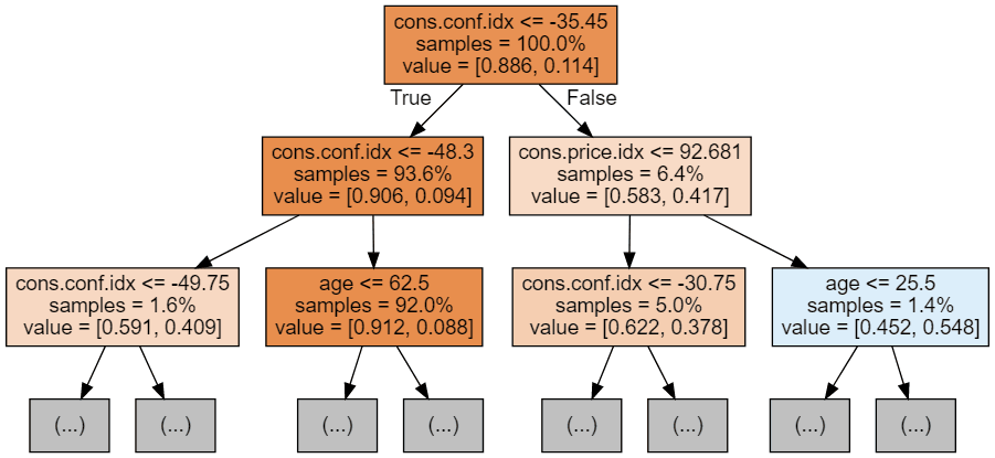
Each tree image is limited to only showing the first few nodes. These trees can get very large and difficult to visualize. The colors represent the majority class of each node (box, with red indicating majority 0 (no subscription) and blue indicating majority 1 (subscription). The colors get darker the closer the node gets to being fully 0 or 1. Each node also contains the following information:

1. The variable name and value used for splitting
2. The % of total samples in each split
3. The % split between classes in each split

Hyperparameter Tuning

The code below uses Scikit-Learn’s RandomizedSearchCV, which will randomly search parameters within a range per hyperparameter. We define the hyperparameters to use and their ranges in the param_dist dictionary. In our case, we are using:

• n_estimators: the number of decision trees in the forest. Increasing this hyperparameter generally improves the performance of the model but also increases the computational cost of training and predicting.
• max_depth: the maximum depth of each decision tree in the forest. Setting a higher value for max_depth can lead to overfitting while setting it too low can lead to underfitting.

param_dist = {'n_estimators': randint(50,500),
              'max_depth': randint(1,20)}

# Create a random forest classifier
rf = RandomForestClassifier()

# Use random search to find the best hyperparameters
rand_search = RandomizedSearchCV(rf, 
                                 param_distributions = param_dist, 
                                 n_iter=5, 
                                 cv=5)

# Fit the random search object to the data
rand_search.fit(X_train, y_train)

RandomizedSearchCV will train many models (defined by n_iter_ and save each one as variables, the code below creates a variable for the best model and prints the hyperparameters. In this case, we haven’t passed a scoring system to the function, so it defaults to accuracy. This function also uses cross validation, which means it splits the data into five equal-sized groups and uses 4 to train and 1 to test the result. It will loop through each group and give an accuracy score, which is averaged to find the best model.

# Create a variable for the best model
best_rf = rand_search.best_estimator_

# Print the best hyperparameters
print('Best hyperparameters:',  rand_search.best_params_)

Output:

Best hyperparameters: {'max_depth': 5, 'n_estimators': 260}

More Random Forest Evaluation Metrics

Let’s look at the confusion matrix. This plots what the model predicted against what the correct prediction was. We can use this to understand the tradeoff between false positives (top right) and false negatives (bottom left). We can plot the confusion matrix using this code:

# Generate predictions with the best model
y_pred = best_rf.predict(X_test)

# Create the confusion matrix
cm = confusion_matrix(y_test, y_pred)

ConfusionMatrixDisplay(confusion_matrix=cm).plot();

Output:

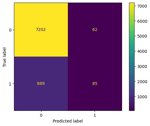
Random forest classifier evaluation using a confusion matrix. Image by Author

We should also evaluate the best model with accuracy, precision, and recall (note your results may differ due to randomization)

y_pred = knn.predict(X_test)

accuracy = accuracy_score(y_test, y_pred)
precision = precision_score(y_test, y_pred)
recall = recall_score(y_test, y_pred)

print("Accuracy:", accuracy)
print("Precision:", precision)
print("Recall:", recall)

Output:

Accuracy: 0.885

Precision: 0.578

Recall: 0.0873

The below code plots the importance of each feature, using the model’s internal score to find the best way to split the data within each decision tree.

# Create a series containing feature importances from the model and feature names from the training data
feature_importances = pd.Series(best_rf.feature_importances_, index=X_train.columns).sort_values(ascending=False)

# Plot a simple bar chart
feature_importances.plot.bar();

This tells us that the consumer confidence index, at the time of the call, was the biggest predictor of whether the person subscribed.

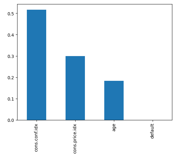
Random forest classifier features in order of importance. Image by Author

Take it to the Next Level

To get started with supervised machine learning in Python, take Supervised Learning with scikit-learn. To learn more about using random forests and other tree-based machine learning models, look at our Machine Learning with Tree-Based Models in Python and Ensemble Methods in Python courses.