Pandas GroupBy Explained: Syntax, Examples, and Tips

Data analysis often requires examining patterns within subsets of your data. If you're calculating average sales by region, analyzing customer behavior by demographics, or aggregating scientific measurements by experimental conditions, then pandas groupby() helps us for efficient data summarization and insights extraction.

In this tutorial, we’ll look at several pandas groupby() operations, from basic syntax to advanced techniques. We’ll also look at the powerful split-apply-combine strategy to transform complex datasets into actionable insights, making you more productive and confident in your data analysis workflow.

What Is Pandas GroupBy?

The pandas groupby() function is a powerful method for organizing data. It works by grouping rows from a DataFrame that share a common value or characteristic into distinct categories. This process is a fundamental step in many Data Manipulation with pandas workflows. 

Its significance lies in its ability to segment large datasets for summary statistics, making it invaluable in finance for portfolio analysis, in scientific research for comparing experimental groups, and in business intelligence for tracking performance metrics.

How Does Pandas GroupBy Work?

The mechanics behind pandas groupby() operations follow a systematic three-phase approach that transforms complex data into meaningful insights. It implements the split-apply-combine strategy.

First, it splits your DataFrame into distinct groups based on specified criteria. Second, it applies functions (aggregations, transformations, or filters) to each group independently. Finally, it combines the results into a unified output structure.

This approach mirrors SQL's GROUP BY functionality but provides superior flexibility for Python workflows. While SQL GROUP BY primarily focuses on aggregation, pandas groupby() supports diverse operations, including data transformation, filtering, and complex statistical computations. 

The result is a powerful tool for extracting insights from complex datasets, enabling analysts to uncover patterns that would be difficult to detect in ungrouped data.

Prerequisites

Before looking into pandas groupby() operations, ensure you have the foundational knowledge and tools necessary for effective learning.

You should be comfortable with basic Python programming concepts and have hands-on experience with pandas DataFrames, including data loading, indexing, and basic operations. Familiarity with NumPy arrays and Python data structures (lists, dictionaries) will enhance your understanding of advanced groupby techniques.

Required Setup

import pandas as pd
import numpy as np
import matplotlib.pyplot as plt

# Verify pandas version (2.0+ recommended)
print(f"Pandas version: {pd.__version__}")

For comprehensive pandas fundamentals, review our Pandas Cheat Sheet: Data Wrangling in Python. 

Pandas GroupBy: Syntax and Parameters

Understanding the complete syntax and parameters of groupby() is essential for leveraging its full potential in data analysis workflows. Let’s look at the syntax and the parameters that this method takes.

Syntax overview

The basic groupby() syntax follows a straightforward pattern that integrates seamlessly into pandas' method chaining approach, as shown below:

df.groupby(by=None, axis=0, level=None, as_index=True, 
           sort=True, group_keys=True, dropna=True)

This method returns a GroupBy object that can be further manipulated with aggregation, transformation, or filtering operations:

# Basic groupby workflow
grouped = df.groupby('column_name')
result = grouped.agg({'numeric_col': 'mean', 'other_col': 'sum'})

Parameter details

Each groupby() parameter controls specific aspects of the grouping behavior, enabling precise control over your data analysis workflow.

• by: The primary grouping criterion - accepts single/multiple columns, functions, or mappings:
• axis: Specifies grouping direction (0=rows, 1=columns). Default is 0 for row-wise grouping.
• level: Groups by specific MultiIndex levels when working with hierarchical data structures.
• as_index: Controls whether group keys become the result index (True) or remain as columns (False).
• sort: Determines if groups are sorted by keys (True) or maintain original order (False) - impacts performance.
• group_keys: Includes group keys in the result when applying functions (True) or omits them (False).
• dropna: Excludes groups with NaN values (True) or includes them (False).

For advanced parameter usage, explore our Reshaping Data with pandas course.

Return value

The groupby() method returns a GroupBy object, not a DataFrame, which serves as an intermediate container for subsequent operations.

This object enables efficient lazy evaluation. Groups are created only when operations are applied, optimizing memory usage for large datasets. The GroupBy object supports method chaining for complex analytical workflows.

The Split-Apply-Combine Mechanism

This object acts as a lightweight container for grouping instructions. When you call groupby(), pandas immediately builds an internal mapping of group labels to row indices. 

However, no actual computation (like aggregation, transformation, or filtering) is performed until you apply a method. This design avoids unnecessary work and allows you to chain methods for complex analytical workflows.

import pandas as pd
import numpy as np

# Create a sample DataFrame
data = {'Team': ['Marketing', 'Sales', 'Sales', 'HR', 'Marketing', 'HR'],
        'Employee': ['Alice', 'Bob', 'Charlie', 'David', 'Eve', 'Frank'],
        'Salary': [90000, 110000, 105000, 75000, 95000, 80000],
        'Projects': [3, 5, 4, 2, 4, 3]}
df = pd.DataFrame(data)

Splitting phase

The first step is splitting. Pandas takes the original DataFrame and partitions it into smaller DataFrames based on the criteria you provide in the by parameter. Each of these smaller DataFrames contains rows that share the same value for the specified key(s).

For our example df, if we group by the 'Team' column (df.groupby('Team')), pandas will create three groups: one for 'Marketing', one for 'Sales', and one for 'HR'. Internally, it creates a dictionary-like structure where the keys are the group names ('Marketing', 'Sales', 'HR') and the values are the row indices belonging to each group.

Performance parameters like sort=False can speed this up by not ordering the group keys, and dropna=False will create a separate group for any NaN values in the grouping column.

Applying phase

Next is the Applying phase. A function or operation is applied independently to each of the smaller DataFrames created in the splitting phase. This is where the actual computation happens. The operations fall into three main categories:

1. Aggregation: Computes a summary statistic for each group, like the mean, sum, or count. This reduces the data to a single value per group. For example, calculating the average salary for each team.
2. Transformation: Performs a group-specific calculation but returns a new series or DataFrame with the same shape as the original group. A common use case is standardizing data within a group (e.g., calculating a z-score). This is useful for feature engineering and is a core concept in reshaping data with pandas.
3. Filtration: Removes entire groups based on a computed property. For example, you could keep only the teams with an average salary above a certain threshold.

While you can use custom functions with the .apply() method, pandas' built-in aggregation functions (.sum(), .mean(), etc.) are highly optimized in Cython and are significantly faster.

Combining phase

Finally, the Combining phase takes the results from the applying phase and stitches them back together into a single pandas object (a DataFrame or Series). The structure of this final object depends on the operation you applied. 

For aggregations, you'll typically get a new DataFrame where the group keys form the index. For transformations, the output will have the same index as your original DataFrame. This final step presents the insights in a clean, organized format.

Key GroupBy Methods and Operations

Building on the split-apply-combine mechanism, pandas offers a suite of methods to perform aggregations, transformations, filtrations, and more on grouped data, enabling sophisticated analyses with minimal code. Now, we’ll look at these key operations, complete with examples, to help you apply groupby() effectively in your data workflows.

Aggregation methods

Aggregation methods summarize each group into a single value or set of values, making them ideal for computing statistics like totals, averages, or counts. Built-in functions such as sum(), mean(), count(), min(), max(), std(), and var() are optimized for performance and cover common use cases, such as calculating team performance metrics in sports data or sales totals by region in business reports.

For custom or multiple aggregations, the agg() method (or its alias aggregate()) provides flexibility. You can pass a dictionary mapping columns to functions, a list of functions for all columns, or even custom lambdas for tailored computations.

Consider this sample DataFrame for demonstrations throughout this section:

import pandas as pd
df = pd.DataFrame({
    'team': ['A', 'A', 'B', 'B', 'C', 'C'],
    'points': [25, 12, 15, 14, 19, 23],
    'assists': [5, 7, 7, 9, 12, 9],
    'rebounds': [11, 8, 10, 6, 6, 5]
})

Using built-in aggregation:

grouped = df.groupby('team')
print(grouped.sum())

Output:

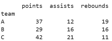
For multiple and custom aggregations:

print(grouped.agg({
    'points': 'sum',
    'assists': 'mean',
    'rebounds': lambda x: x.max() - x.min()
}))

Output:

This approach is particularly useful in exploratory data analysis; for a broader overview of your dataset before grouping, try Pandas Profiling (ydata-profiling) in Python: A Guide for Beginners

Transformation methods

Transformation methods apply functions to each group and return a result with the same shape as the original data, preserving the index for easy reintegration. They're beneficial in scenarios like group-wise normalization (to compare within categories), imputation (filling missing values based on group statistics), or scaling features for machine learning.

Practical examples include standardizing scores per team or filling NaNs with group medians. The transform() method is key here, supporting built-in functions or custom lambdas.

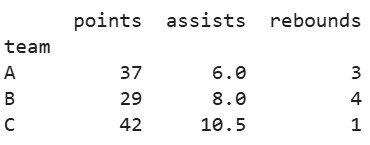
Example of normalization (z-score per group for 'points'):

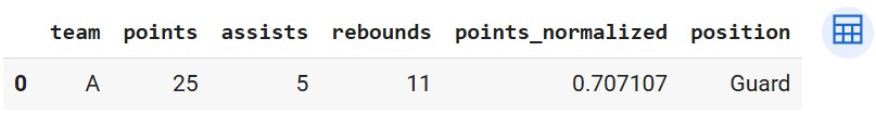
df['points_normalized'] = grouped['points'].transform(lambda x: (x - x.mean()) / x.std())
print(df)

Output:

This technique ensures fair comparisons across groups with different scales. For more on applying custom functions, see the Pandas Apply Tutorial.

Filtration methods

Filtration allows you to selectively include or exclude entire groups based on conditions evaluated on the group as a whole, which is perfect for focusing on subsets like high-performing teams or removing small sample sizes to avoid bias. 

The filter() method takes a function that returns a boolean for each group. If True, the group's rows are kept in the output DataFrame.

Predicates are evaluated once per group, often using aggregates like len(x) > n for size or x['column'].sum() > threshold for sums. This is efficient as it avoids row-by-row checks.

Example: Filter teams with total points over 30

filtered = grouped.filter(lambda x: x['points'].sum() > 30)
print(filtered)

Output:

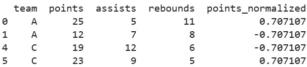
Here, team B (29 points) is excluded. During data cleaning, combine this with techniques from the Pandas Drop Duplicates Tutorial to handle redundancies post-filtration.

Getting group sizes and indices

Understanding group composition is crucial for validation and debugging; pandas provides methods to count groups, get sizes, and retrieve specific subgroups. Use ngroups for the total number of groups, size() for a Series of group sizes, and get_group(key) to access a particular group's DataFrame.

Example:

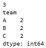
print(len(grouped))  # Number of groups: 3
print(grouped.size())

Output:

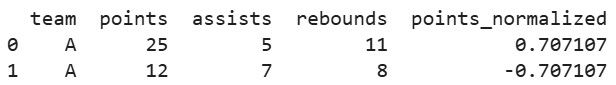
print(grouped.get_group('A'))

Output:

These are handy for iterative analysis, where group sizes inform clustering validity.

Working with multiple columns

Grouping by multiple columns creates hierarchical (multi-index) groups, enabling nuanced analysis like performance by team and position. Specify a list in by, and the result will have a MultiIndex unless as_index=False.

Handling hierarchical results involves methods like reset_index() for flattening or xs() for cross-sections. For deeper insights, take a look at Hierarchical indices, groupby, and pandas.

Let’s add a 'position' column for this example:

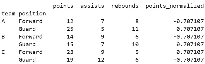
df['position'] = ['Guard', 'Forward', 'Guard', 'Forward', 'Guard', 'Forward']
multi_grouped = df.groupby(['team', 'position'])
print(multi_grouped.sum())

Output:

Now, let’s query multiple parameters in the group

multi_grouped.get_group(('A', 'Guard'))

Output:

Pandas GroupBy Examples

In the previous section, we’ve looked at different methods of pandas groupby(). Let's apply these concepts through hands-on examples ranging from basic to advanced scenarios. These demonstrations use synthetic datasets inspired by real-world data, illustrating how groupby() can transform raw information into meaningful insights.

Example 1: Grouping by a single column

Start with a straightforward case: grouping a dataset by a single column to compute basic aggregates. This is common in initial exploratory analysis, such as summarizing sales by product category.

Using a simple sales DataFrame:

import pandas as pd

data = {
    'product': ['Laptop', 'Phone', 'Laptop', 'Tablet', 'Phone', 'Tablet'],
    'sales': [1200, 800, 1500, 600, 900, 700],
    'region': ['East', 'West', 'East', 'West', 'East', 'West']
}
df = pd.DataFrame(data)

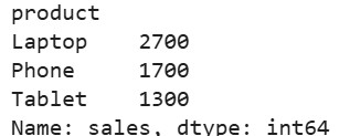
# Group by 'product' and aggregate sales with sum and mean
grouped = df.groupby('product')
agg_result = grouped['sales'].agg(['sum', 'mean'])
print(agg_result)

Output:

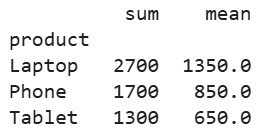
This reveals total and average sales per product, helping identify top performers.

Example 2: Grouping by multiple columns

For deeper analysis, group by multiple columns to create hierarchical structures, such as sales by product and region. This uncovers regional variations within categories.

Extending the previous DataFrame:

multi_grouped = df.groupby(['product', 'region'])
multi_agg = multi_grouped['sales'].sum()
print(multi_agg)

Output:

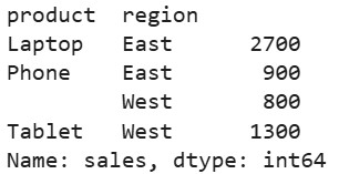
The result is a Series with a MultiIndex, allowing queries like multi_agg.loc['Laptop'] to focus on specifics. This technique is invaluable for segmented reporting.

Example 3: Aggregating multiple columns

Aggregate different columns with varied functions to get a comprehensive view, such as summing sales while averaging other metrics.

Let’s add a 'units' column to the DataFrame:

df['units'] = [5, 10, 6, 8, 12, 9]

# Group by 'product' and apply different aggregations
agg_multi_col = df.groupby('product').agg({
    'sales': 'sum',
    'units': 'mean'
})
print(agg_multi_col)

Output:

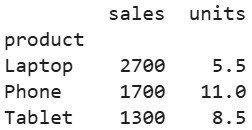
This provides a multifaceted summary, useful for inventory planning alongside revenue tracking.

Example 4: Real-world dataset example

Let's apply groupby() to an air quality dataset mimicking real-world environmental monitoring (inspired by public sources like EPA air quality indexes). This end-to-end workflow covers data loading, grouping, aggregation, and insight extraction, such as analyzing pollutant levels by city and date. 

First, create the dataset (in practice, you'd load from a CSV. Here, we simulate for demonstration):

import pandas as pd
import numpy as np

# Synthetic air quality data
dates = pd.date_range(start='2023-01-01', periods=12, freq='ME')
cities = ['New York', 'Los Angeles', 'Chicago']
data = {
    'date': np.repeat(dates, len(cities)),
    'city': np.tile(cities, len(dates)),
    'pm25': np.random.uniform(5, 50, len(dates)*len(cities)),  # Particulate matter
    'o3': np.random.uniform(20, 100, len(dates)*len(cities))   # Ozone
}
aq_df = pd.DataFrame(data)

# Group by 'city' and aggregate means
city_grouped = aq_df.groupby('city').agg({
    'pm25': 'mean',
    'o3': 'mean'
})
print(city_grouped)

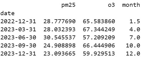
# Further, group by month across all cities
aq_df['month'] = aq_df['date'].dt.month
month_grouped = aq_df.groupby('month').agg({
    'pm25': 'max',
    'o3': 'min'
})
print(month_grouped)

Output:

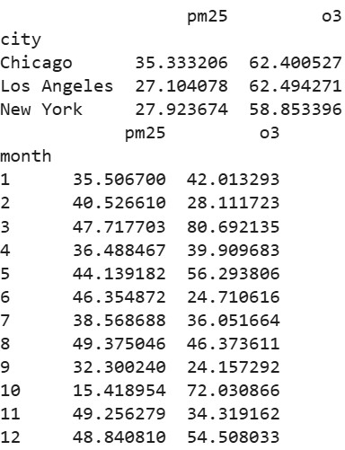
Insights: Higher PM2.5 in Chicago suggests urban pollution trends and monthly maxes highlight seasonal peaks. You can explore more like this analysis in this course - Analyzing Police Activity with pandas.

Using Lambda functions in groupby

Lambda functions enable custom logic within groupby(), ideal for ad-hoc calculations not covered by built-ins, such as range computation per group.

Let’s see an example of this using the air quality DataFrame from the previous example:

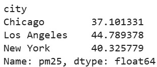
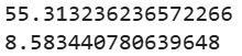
# Custom lambda to calculate range (max - min) for pm25 per city
range_pm25 = aq_df.groupby('city')['pm25'].agg(lambda x: x.max() - x.min())
print(range_pm25)

Output:

For more complex custom applications, take a look at the Pandas Apply Tutorial

Hierarchical indexes

Multi-column grouping naturally creates hierarchical indexes, which organize data in levels for efficient slicing. To work with them, use loc with tuples or reset_index() to flatten.

From the multi-grouped sales example earlier:

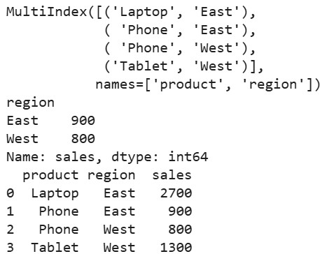
# Assuming multi_agg from Example 2
print(multi_agg.index)  # MultiIndex([('Laptop', 'East'), ...])

# Slice by level
print(multi_agg.loc['Phone'])

# Flatten
flat_df = multi_agg.reset_index()
print(flat_df)

Output:

To learn more about these concepts, take a look at Hierarchical indices, groupby, and pandas.

Resampling and time-based grouping

For temporal data, use pd.Grouper or resample() with groupby() to aggregate by time intervals, like monthly averages in a time series.

Let’s take a look at an example using the air quality DataFrame (set 'date' as index for resampling) from the earlier example:

aq_df.set_index('date', inplace=True)

# Resample monthly and mean (across all cities)
monthly_resampled = aq_df.resample('M').mean(numeric_only=True)
print(monthly_resampled)

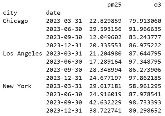
# Alternatively, group by city and month with Grouper
aq_df.reset_index(inplace=True)  # Reset for grouping
time_grouped = aq_df.groupby(['city', pd.Grouper(key='date', freq='M')]).mean(numeric_only=True)
print(time_grouped)

This is important for trend analysis.

Advanced Grouping Techniques

So far, we’ve seen basic groupby() applications. Knowing advanced techniques can unlock even more efficiency and insight, particularly for specialized data types like time series or categorical variables. So let’s look at some time-based and categorical grouping, offering strategies to handle temporal patterns and optimize performance in large-scale analyses, building on the examples we've seen so far.

Time-based grouping

Time-based grouping is essential for analyzing datasets with datetime components, such as financial time series or sensor logs, allowing you to bin data into intervals like days, months, or custom frequencies. Using pd.Grouper within groupby() or the resample() method on datetime-indexed DataFrames, you can aggregate over time windows with parameters for frequency, closed sides, labels, and offsets to fine-tune binning.

Building on the air quality dataset from earlier examples, let's look at advanced time binning. Assume we've loaded the DataFrame aq_df with 'date' as a datetime column:

import pandas as pd

# Assuming aq_df from previous example, with 'date' as datetime
# Group by city and quarterly time bins using Grouper
quarterly_grouped = aq_df.groupby(['city', pd.Grouper(key='date', freq='Q')]).agg({
    'pm25': 'mean',
    'o3': 'max'
})
print(quarterly_grouped)

Output:

Relevant parameters include freq (e.g., 'W' for weekly, '2M' for bimonthly), closed ('left' or 'right' to specify bin edge inclusion), label ('left' or 'right' for timestamp labeling), and origin for custom starting points. For offsets, use pd.offsets.BusinessDay() in freq for business-aware grouping.

With resample() on a datetime index:

aq_df.set_index('date', inplace=True)
# Resample quarterly, with custom parameters
quarterly_resampled = aq_df.resample('Q', closed='left', label='left').mean(numeric_only=True)
print(quarterly_resampled)

Output:

This is particularly powerful for trend detection in datasets like stock prices or weather records. For more on handling time series, check out Pandas Resample With resample() and asfreq() and stay updated with features from Pandas 2.0: What’s New and Top Tips.

Categorical grouping

Converting grouping columns to pandas' categorical dtype before groupby() can significantly enhance performance and memory usage, especially for datasets with repetitive string or integer values like categories or labels. These advantages include a smaller memory footprint (achieved by storing unique values internally), quicker operations through optimized hashing, and improved management of ordered categories for sorting or comparisons..

To convert, use astype('category'), which is ideal for columns with low cardinality (few unique values relative to rows). Let’s see this using the sales DataFrame from earlier examples:

# Convert 'product' to category
df['product'] = df['product'].astype('category')

# Now group: operations are faster
cat_grouped = df.groupby('product')
print(cat_grouped['sales'].sum())

Output:

Benchmarking on a large DataFrame (e.g., 1 million rows with 10 unique products), categorical grouping can reduce memory by up to 90% and speed up aggregation by 2-5x compared to object dtype strings. This optimization is useful in memory-constrained environments or when chaining with other operations.

For ordered categories, set ordered=True during conversion to enable natural sorting or range-based queries. If you're learning pandas comprehensively, resources like How to Learn pandas cover these dtypes in depth.

Tips, Performance, and Best Practices

To effectively implement pandas groupby() and optimize your data analysis, we need to focus on performance enhancements and best practices, especially with large, complex datasets. So let’s look at some ways to accelerate operations, manage resources effectively, and prevent common mistakes, ensuring your analyses are reliable and scalable for real-world use.

Improving groupby performance

Speeding up groupby() operations can make a significant difference in iterative workflows, particularly with large DataFrames where computation time adds up. Prioritize built-in aggregation methods like sum() or mean() over custom functions via apply() or lambdas, as the former are vectorized and leverage Cython-optimized code for faster execution. 

For instance, on a million-row dataset, using grouped.sum() might take seconds, while an equivalent lambda could double that time. Avoid unnecessary computations by selecting only relevant columns before grouping with df[['key', 'value']].groupby('key'), reducing the data processed. Set sort=False if order doesn't matter, and use observed=True for categorical groups to skip unseen categories. 

Memory management

Efficient memory usage prevents out-of-memory errors and allows handling larger datasets on standard hardware. Select only necessary columns early (df.groupby('key')[['col1', 'col2']]), and convert grouping keys to categoricals as discussed in advanced techniques to compress storage potentially reducing usage by 50-90% for string-heavy columns.

Downcast numeric types with pd.to_numeric(df['col'], downcast='float') or use sparse DataFrames for datasets with many zeros. Monitor memory with df.memory_usage(deep=True)before and after optimizations. Let’s see this with an example:

import pandas as pd 
import numpy as np 

# Large sample DataFrame 
df_large = pd.DataFrame({ 'category': np.random.choice(['A', 'B', 'C'], size=1000000), 'value': np.random.randn(1000000) }) 

# Before optimization 
print(df_large.memory_usage(deep=True).sum() / 1024**2) 

# Convert to categorical 
df_large['category'] = df_large['category'].astype('category') print(df_large.memory_usage(deep=True).sum() / 1024**2)

Output:

Working with large datasets

For datasets exceeding memory limits, scale beyond pandas with libraries like Dask, which parallelizes groupby() across cores or clusters using a similar API, or process in chunks via pd.read_csv(chunksize=n) and aggregate incrementally.

With Dask:

import dask.dataframe as dd

# Load large CSV in chunks
ddf = dd.read_csv('large_file.csv')
grouped_dask = ddf.groupby('category').sum().compute()  # Compute to execute

This handles gigabyte-scale data lazily. 

Alternatively, for chunking in pure pandas:

chunks = pd.read_csv('large_file.csv', chunksize=100000)
agg_results = []
for chunk in chunks:
    agg_results.append(chunk.groupby('category').sum())
final_agg = pd.concat(agg_results).groupby(level=0).sum()

Common pitfalls

Typical mistakes include forgetting to handle NaNs (use dropna=False if needed), misusing as_index=False leading to unexpected outputs, or applying apply() inefficiently on large groups. To mitigate this opt for agg() or transform() instead. 

Another is ignoring MultiIndex complexities after multi-column grouping. Always use reset_index() if flattening is required to avoid indexing errors. Debug by inspecting the GroupBy object with grouped.groups or grouped.ngroups. 

When to use groupby

Groupby() works best in scenarios requiring category based summaries, like cohort analysis in marketing or per-sensor averages in IoT data, where it outperforms manual loops or pivot tables for flexibility. 

However, for simple pivots, consider pd.pivot_table(). For row-wise operations without grouping, use apply() directly and for very large distributed data, migrate to Spark or Dask early.

Common Pandas GroupBy Use Cases

Pandas groupby() works well in diverse domains by enabling targeted data summarization and manipulation. This makes it a versatile tool for extracting value from structured data. It has several practical applications in business, science, and data preparation. Let’s look at some of those.

Business analytics

In business analytics, groupby() facilitates quick insights into performance metrics, customer behavior, and operational trends, such as segmenting sales data by demographics or time periods to inform strategies. 

For example, analysts might group transaction data by customer segments to calculate lifetime value or by product lines to identify top revenue drivers, supporting inventory management and marketing campaigns.

Consider a retail dataset for quarterly sales analysis:

import pandas as pd

# Sample business data
data = {
    'quarter': ['Q1', 'Q1', 'Q2', 'Q2', 'Q3', 'Q3'],
    'product': ['Widget A', 'Widget B', 'Widget A', 'Widget B', 'Widget A', 'Widget B'],
    'revenue': [50000, 30000, 60000, 40000, 55000, 35000],
    'units_sold': [1000, 600, 1200, 800, 1100, 700]
}
biz_df = pd.DataFrame(data)

# Group by quarter and product, aggregate revenue and average units
biz_grouped = biz_df.groupby(['quarter', 'product']).agg({
    'revenue': 'sum',
    'units_sold': 'mean'
})
print(biz_grouped)

Output:

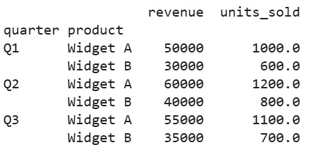
This reveals growth patterns, like increasing Widget A revenue from Q1 to Q2, guiding budgeting. For joining such data with external sources, explore Joining Data with pandas.

Scientific data processing

In scientific research and experimentation, groupby() aggregates results by variables like treatment groups or measurement conditions, enabling statistical comparisons and hypothesis testing in fields like biology or physics. It's commonly used to compute means and variances per experimental batch or to summarize sensor readings by time intervals, aiding in pattern detection and reproducibility.

Let’s look at an example to see this in action.

import pandas as pd
import numpy as np

# Synthetic penguin data
data = {
    'species': ['Adelie', 'Adelie', 'Gentoo', 'Gentoo', 'Chinstrap', 'Chinstrap'],
    'island': ['Torgersen', 'Biscoe', 'Biscoe', 'Dream', 'Dream', 'Torgersen'],
    'bill_length_mm': [39.1, 37.8, 46.1, 47.3, 46.5, 50.0],
    'body_mass_g': [3750, 3450, 5075, 4875, 3500, 3900]
}
penguin_df = pd.DataFrame(data)

# Group by species, compute mean and std for measurements
sci_grouped = penguin_df.groupby('species').agg({
    'bill_length_mm': ['mean', 'std'],
    'body_mass_g': ['mean', 'std']
})
print(sci_grouped)

Output:

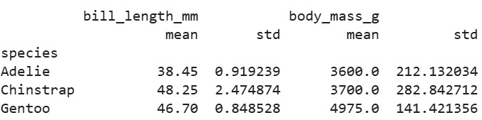
This highlights species differences, useful for clustering or further analysis with tools like numpy for advanced stats.

Data cleaning and preprocessing

Groupby() aids data cleaning by enabling group-wise operations like deduplication, outlier detection, and imputation, ensuring high-quality inputs for modeling. For deduplication, group by key columns and filter uniques. For outliers, it transforms the flag values beyond group thresholds and for imputation, fill NaNs with group medians to preserve subgroup characteristics.

Example with a dataset containing duplicates and missing values:

import pandas as pd
import numpy as np

# Sample data with issues
data = {
    'id': [1, 1, 2, 2, 3, 3],
    'group': ['X', 'X', 'Y', 'Y', 'Z', 'Z'],
    'value': [10, 10, 20, np.nan, 30, 25]
}
clean_df = pd.DataFrame(data)

# Deduplicate by group and id
deduped = clean_df.groupby(['group', 'id']).first().reset_index()

# Impute missing values with group median
clean_df['value'] = clean_df.groupby('group')['value'].transform(lambda x: x.fillna(x.median()))

# Detect outliers (e.g., > 2 std from group mean)
clean_df['outlier'] = clean_df.groupby('group')['value'].transform(lambda x: np.abs(x - x.mean()) > 2 * x.std())

print(clean_df)

Output:

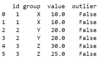
This preprocesses data effectively.

Conclusion

Throughout this comprehensive tutorial, we've looked at the fundamentals of pandas groupby()its definition, syntax, and the split-apply-combine mechanism and advanced techniques like time-based and categorical grouping, complete with practical examples, performance tips, and real-world use cases.

As you integrate these concepts into your data science toolkit, remember that proficiency comes with practice. Experiment with your own datasets, perhaps starting with projects like analyzing public datasets or building dashboards, to deepen your expertise.

If you're eager to further develop your data science skills, I recommend taking the Data Scientist in Python career track, which covers everything you need to know to kick start your career.