Course
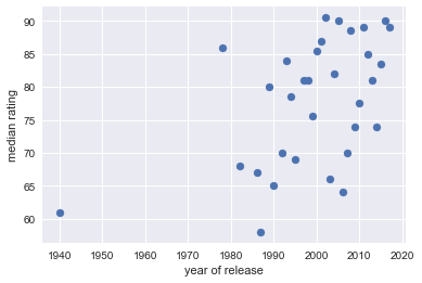
In a previous post, you saw how the groupby operation arises naturally through the lens of the principle of split-apply-combine. You checked out a dataset of Netflix user ratings and grouped the rows by the release year of the movie to generate the following figure:

This was achieved via grouping by a single column. I mentioned, in passing, that you may want to group by several columns, in which case the resulting pandas DataFrame ends up with a multi-index or hierarchical index. In this post, you'll learn what hierarchical indices and see how they arise when grouping by several features of your data. You can find out more about all of these concept and practices in our Manipulating DataFrames with pandas course.
So first up: what are hierarchical indices?

Hierarchical Indices and pandas DataFrames
What is the Index of a DataFrame?
Before introducing hierarchical indices, I want you to recall what the index of pandas DataFrame is. The index of a DataFrame is a set that consists of a label for each row. Let's look at an example. I'll first import a synthetic dataset of a hypothetical DataCamp student Ellie's activity on DataCamp. The columns are a date, a programming language and the number of exercises that Ellie completed that day in that language. Load in the data:
# Import pandas
import pandas as pd

# Load in data
df = pd.read_csv('data/user_ex_python.csv')
df
Run and edit the code from this tutorial online
Run code| date | language | ex_complete | |
|---|---|---|---|
| 0 | 2017-01-01 | python | 6 |
| 1 | 2017-01-02 | python | 5 |
| 2 | 2017-01-03 | python | 10 |
You can see the Index on the left hand side of the DataFrame and that it consists of integers. This is a RangeIndex:
# Check out index
df.index
RangeIndex(start=0, stop=3, step=1)
We can use this index to slice out a row or rows of df:
# Slice and dice data
df.loc[:1]
| date | language | ex_complete | |
|---|---|---|---|
| 0 | 2017-01-01 | python | 6 |
| 1 | 2017-01-02 | python | 5 |
This index, however, is not so informative. If you're going to label the rows of your DataFrame, it would be good to label them in a meaningful manner, if at all possible. Can you do this with the dataset in question? A good way to think about this challenge is that you want a unique and meaningful identifier for each row. Check out the columns and see if any matches these criteria. Notice that the date column contains unique dates so it makes sense to label each row by the date column. That is,you can make the date column the index of the DataFrame using the .set_index() method (n.b. inplace=True means you're actually altering the DataFrame df inplace):
# Set new index
df.set_index(pd.DatetimeIndex(df['date']), inplace=True)
df
| date | language | ex_complete | |
|---|---|---|---|
| date | |||
| 2017-01-01 | 2017-01-01 | python | 6 |
| 2017-01-02 | 2017-01-02 | python | 5 |
| 2017-01-03 | 2017-01-03 | python | 10 |
This then gives df a DateTimeIndex:
# Check out new index
df.index
DatetimeIndex(['2017-01-01', '2017-01-02', '2017-01-03'], dtype='datetime64[ns]', name='date', freq=None)
Now you can slice out rows using the DateTimeIndex that you've created:
# Slice and dice data w/ new index
df.loc['2017-01-02']
date           2017-01-02
language           python
ex_complete             5
Name: 2017-01-02 00:00:00, dtype: object
Also note that the .columns attribute returns an index containg the column names of df:
# Check out columns
df.columns
Index(['date', 'language', 'ex_complete'], dtype='object')
This can be slightly confusing because this says is that df.columns is of type Index. This does not mean that the columns are the index of the DataFrame. The index of df is always given by df.index. Check out our pandas DataFrames tutorial for more on indices. Now it's time to meet hierarchical indices.
The Multi-index of a pandas DataFrame
What if we had multiple languages for our dataset, as we do on DataCamp? Have a look:
# Import and check out data
df = pd.read_csv('data/user_ex.csv')
df
| date | language | ex_complete | |
|---|---|---|---|
| 0 | 2017-01-01 | python | 6 |
| 1 | 2017-01-02 | python | 5 |
| 2 | 2017-01-03 | python | 10 |
| 3 | 2017-01-01 | r | 8 |
| 4 | 2017-01-02 | r | 8 |
| 5 | 2017-01-03 | r | 8 |
Each date now corresponds to several rows, one for each language. See, for example, that the date '2017-01-02' occurs in rows 1 and 4, for languages Python and R, respectively. Thus the date no longer uniquely specifies the row. However, 'date' and 'language' together do uniquely specify the rows. For this reason, we use both as the index:
# Set index
df.set_index(['date', 'language'], inplace=True)
df
| ex_complete | ||
|---|---|---|
| date | language | |
| 2017-01-01 | python | 6 |
| 2017-01-02 | python | 5 |
| 2017-01-03 | python | 10 |
| 2017-01-01 | r | 8 |
| 2017-01-02 | r | 8 |
| 2017-01-03 | r | 8 |
You have now created a multi-index, or hierarchical index (become comfortable with both these terms as you'll find them used interchangeably), and you can see this by checking out the index as follows:
# Check out multi-index
df.index
MultiIndex(levels=[['2017-01-01', '2017-01-02', '2017-01-03'], ['python', 'r']],
           labels=[[0, 1, 2, 0, 1, 2], [0, 0, 0, 1, 1, 1]],
           names=['date', 'language'])
The above tells you that your DataFrame df now has a MultiIndex with two levels, the first given by the date, the second by the the language. Recall that above you were able to slice the DataFrame using the index and the .loc accessor: df.loc['2017-01-02']. To be able to slice with a multi-index, you need to sort the index first:
# Sort index
df.sort_index(inplace=True)
df
| ex_complete | ||
|---|---|---|
| date | language | |
| 2017-01-01 | python | 6 |
| r | 8 | |
| 2017-01-02 | python | 5 |
| r | 8 | |
| 2017-01-03 | python | 10 |
| r | 8 |
Now you can slice out the number of R exercises completed on 2017-01-02 by passing a tuple to the .loc accessor:
# Slice & dice your DataFrame
df.loc[('2017-01-02', 'r')]
ex_complete    8
Name: (2017-01-02, r), dtype: int64
When and why to use multi-indexes
Multi-indexes are a powerful tool for data analysis and organization in pandas. They allow users to create hierarchical indexes, which can be used to group and aggregate data across multiple dimensions. Multi-indexes are particularly useful when working with complex datasets that have multiple levels of categorization, such as financial or time-series data.
By creating a multi-index, users can group data by multiple variables simultaneously, which can reveal insights that might not be apparent from a single-level grouping. For example, multi-indexes can be used to group data by both time and location, allowing analysts to examine trends in specific regions over time.
Additionally, multi-indexes can be used to efficiently select and subset data, as the index provides a convenient way to access specific subsets of the data. Overall, multi-indexes are a powerful tool for organizing, grouping, and analyzing complex datasets in pandas, and are essential for any data analyst or scientist working with hierarchical data.
You now know a bit about hierarchical indices (or multi-indices). It's time to see how they arise when working with groupby objects.
Hierarchical Indices, groupby Objects and Split-Apply-Combine
In a previous post, we explored groupby objects and the data analytic principles of split-apply-combine using netflix data. Lets have a quick refresher with a different dataset, the tips dataset that is built into the seaborn package. 'Tips' contains features such as tip, total_bill, the day of the week and the time of day. First load and explore the data:
# Import and check out data
import seaborn as sns
tips = sns.load_dataset("tips")
tips.head()
| total_bill | tip | sex | smoker | day | time | size | |
|---|---|---|---|---|---|---|---|
| 0 | 16.99 | 1.01 | Female | No | Sun | Dinner | 2 |
| 1 | 10.34 | 1.66 | Male | No | Sun | Dinner | 3 |
| 2 | 21.01 | 3.50 | Male | No | Sun | Dinner | 3 |
| 3 | 23.68 | 3.31 | Male | No | Sun | Dinner | 2 |
| 4 | 24.59 | 3.61 | Female | No | Sun | Dinner | 4 |
Note that the index of tips is a RangeIndex:
# Check out index
tips.index
RangeIndex(start=0, stop=244, step=1)
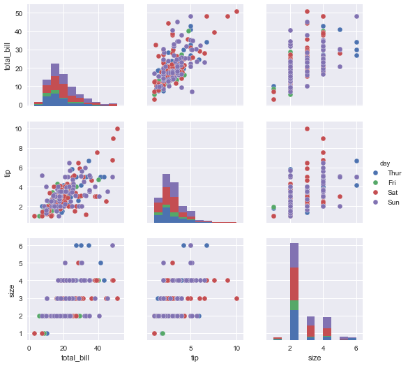
It always helps to do some visual EDA before diving into computation and seaborn's pairplot function allows you to get an overview of all numerical variables:
# Import pyplot, figures inline, set style, plot pairplot
import matplotlib.pyplot as plt
%matplotlib inline
sns.set()
sns.pairplot(tips, hue='day');

If you want to check out how the average tip differs between 'smokers' and 'non-smokers', you can split the original DataFrame by the 'smoker' (using groupby), apply the function 'mean' and combine into a new DataFrame:
# Get mean of smoker/non-smoker groups
df = tips.groupby('smoker').mean()
df
| total_bill | tip | size | |
|---|---|---|---|
| smoker | |||
| Yes | 20.756344 | 3.008710 | 2.408602 |
| No | 19.188278 | 2.991854 | 2.668874 |
The resulting index of the DataFrame df is the 'smoker' column/feature of the original 'tips' DataFrame:
# Check out new index
df.index
CategoricalIndex(['Yes', 'No'], categories=['Yes', 'No'], ordered=False, name='smoker', dtype='category')
If desired, you can reset the index so that 'smoker' becomes a column of the DataFrame:
# Reset the index
df.reset_index()
| smoker | total_bill | tip | size | |
|---|---|---|---|---|
| 0 | Yes | 20.756344 | 3.008710 | 2.408602 |
| 1 | No | 19.188278 | 2.991854 | 2.668874 |
Now it's time to find out how hierarchical indices arise from split-apply-combine and groupby operations.
Multiple groupings and hierarchical indices
Above, you grouped the tips dataset according to the feature 'smoker'. Sometimes you will need to group a dataset according to two features. For example, it is natural to group the tips dataset into smokers/non-smokers & dinner/lunch. To do this, you pass the column names you wish to group by as a list:
# Group by two columns
df = tips.groupby(['smoker','time']).mean()
df
| total_bill | tip | size | ||
|---|---|---|---|---|
| smoker | time | |||
| Yes | Lunch | 17.399130 | 2.834348 | 2.217391 |
| Dinner | 21.859429 | 3.066000 | 2.471429 | |
| No | Lunch | 17.050889 | 2.673778 | 2.511111 |
| Dinner | 20.095660 | 3.126887 | 2.735849 |
Looking at the above, you may be able to see that both 'smoker' and 'time' are indices of df. This is the case and makes sense: if grouping by 'smoker' results in the index being the original 'smoker' column, grouping by two columns will give you two indices. Check the index to confirm that it's hierarchical:
# Check out index
df.index
MultiIndex(levels=[['Yes', 'No'], ['Lunch', 'Dinner']],
           labels=[[0, 0, 1, 1], [0, 1, 0, 1]],
           names=['smoker', 'time'])
And it is. You can do a bunch of useful things now, such as getting the counts in each grouping:
# Group by two features
tips.groupby(['smoker','time']).size()
smoker  time
Yes     Lunch      23
        Dinner     70
No      Lunch      45
        Dinner    106
dtype: int64
You can swap the levels of the hierarchical index also so that 'time' occurs before 'smoker' in the index:
# Swap levels of multi-index
df.swaplevel()
| total_bill | tip | size | ||
|---|---|---|---|---|
| time | smoker | |||
| Lunch | Yes | 17.399130 | 2.834348 | 2.217391 |
| Dinner | Yes | 21.859429 | 3.066000 | 2.471429 |
| Lunch | No | 17.050889 | 2.673778 | 2.511111 |
| Dinner | No | 20.095660 | 3.126887 | 2.735849 |
You may then wish to remove one of these features from the hierarchical index and form different columns with respect to that feature. You can do so using the unstack method:
# Unstack your multi-index
df.unstack()
| total_bill | tip | size | ||||
|---|---|---|---|---|---|---|
| time | Lunch | Dinner | Lunch | Dinner | Lunch | Dinner |
| smoker | ||||||
| Yes | 17.399130 | 21.859429 | 2.834348 | 3.066000 | 2.217391 | 2.471429 |
| No | 17.050889 | 20.095660 | 2.673778 | 3.126887 | 2.511111 | 2.735849 |
You can unstack on the outer feature of the index using the keyword argument 'level':
# Unsstack the outer index
df.unstack(level=0)
| total_bill | tip | size | ||||
|---|---|---|---|---|---|---|
| smoker | Yes | No | Yes | No | Yes | No |
| time | ||||||
| Lunch | 17.399130 | 17.050889 | 2.834348 | 2.673778 | 2.217391 | 2.511111 |
| Dinner | 21.859429 | 20.095660 | 3.066000 | 3.126887 | 2.471429 | 2.735849 |
The result of unstacking has a non-hierarchical index, as you may expect:
# Check out index
df.unstack().index
CategoricalIndex(['Yes', 'No'], categories=['Yes', 'No'], ordered=False, name='smoker', dtype='category')
As a result, you can now perform all types of data analysis with respect to these groupings. I encourage you to do so.
Hierarchical Indices in Daily Use
In this post, you have been introduced to hierarchical indices (or multi-indices) and have seen how they arise as a natural consequence of wanting a DataFrame index to uniquely and meaningfully label the rows of your DataFrame. You have also seen how they arise when you need to group your data by multiple columns, invoking the principle of split-apply-combine. I hope that you have fun with hierarchical indices in your work.
This post was generated from a Jupyter Notebook; You can find it in this repository. If you have any thoughts, responses and/or ruminations, feel free to reach out to me on twitter: @hugobowne.
Check out DataCamp's other handy pandas tutorials, including:


