मैक्लॉरिन श्रेणी: सूत्र, विस्तार, और उदाहरण

कुछ फलन इतने जटिल होते हैं कि उनके साथ सीधे काम करना कठिन पड़ता है — इसलिए गणितज्ञों ने उन्हें बहुपदों से लगभगित करना सीख लिया।

यही मैक्लॉरिन श्रेणी के पीछे का बुनियादी विचार है। यह किसी फलन को बहुपदीय पदों के अनंत योग के रूप में दर्शाती है, जहाँ प्रत्येक पद उस फलन के शून्य पर लिए गए अवकलजों से बनता है। नतीजा ऐसा रूप होता है जिसके साथ आप गणना कर सकें, भले मूल फलन बहुत जटिल हो।

आप मैक्लॉरिन श्रेणी को टेलर श्रेणी का एक खास मामला मान सकते हैं, जो शून्य पर केंद्रित होती है। यह बाधा व्युत्पत्ति को सरल और उपयोग में आसान बना देती है।

इस लेख में, मैं मैक्लॉरिन श्रेणी का सूत्र बताऊँगा, सबसे सामान्य विस्तारों से गुजरूँगा, और उन्हें समझने व लागू करने का तरीका दिखाऊँगा।

मैक्लॉरिन श्रेणी क्या है?

मैक्लॉरिन श्रेणी किसी फलन को उसके शून्य पर लिए गए अवकलजों से बने पदों के अनंत योग के रूप में प्रस्तुत करती है।

प्रत्येक पद एक बहुपद होता है — x की कोई घात जिसे अवकलज के मान से गुणा किया गया है। जब आप ऐसे पर्याप्त पदों को जोड़ते हैं, तो एक बहुपद मिलता है जो मूल फलन जैसा ही आचरण करता है, कम-से-कम शून्य के आसपास।

जटिल फलन को बहुपद से लगभगित करना मैक्लॉरिन श्रेणी का मूल विचार है। बहुपदों की गणना, अवकलन, और समाकलन आसान होते हैं। अधिकांश अन्य फलनों के साथ ऐसा नहीं है।

मैक्लॉरिन श्रेणी बनाम टेलर श्रेणी

टेलर श्रेणी किसी भी बिंदु a पर केंद्रित अनंत बहुपद के रूप में फलन का सन्निकटन देती है। आप बिंदु चुनते हैं, उसके आसपास श्रेणी बनाते हैं, और उस बिंदु के आस-पास अच्छा काम करने वाला बहुपद पाते हैं।

मैक्लॉरिन श्रेणी बस वही टेलर श्रेणी है जहाँ a = 0 होता है। यही एकमात्र अंतर है।

शून्य पर केंद्रित करने से गणित सरल हो जाता है क्योंकि बहुपदीय पदों से (x - a) जैसा अस्थानांतरण हट जाता है और वे साधारण x की घातें बन जाते हैं। कलन, भौतिकी और मशीन लर्निंग में जिन मानक फलनों से आप काम करते हैं, उनके साफ-सुथरे, सुविख्यात मैक्लॉरिन विस्तार इसी वजह से मिलते हैं।

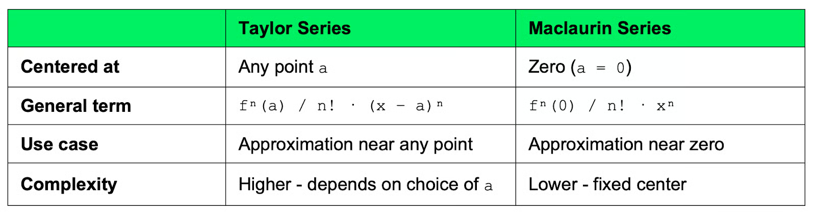
टेलर और मैक्लॉरिन श्रेणी की तुलना

संक्षेप में, जब आपको शून्य के अलावा किसी खास बिंदु के पास सन्निकटन चाहिए तो टेलर श्रेणी का उपयोग करें। जब शून्य आरंभिक बिंदु हो — जो अक्सर होता है — तो मैक्लॉरिन श्रेणी अपनाएँ।

मैक्लॉरिन श्रेणी का सूत्र

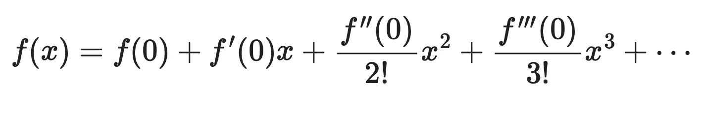
मैक्लॉरिन श्रेणी का सूत्र किसी भी फलन f(x) को अनंत योग के रूप में लिखता है:

मैक्लॉरिन श्रेणी का सूत्र

विस्तारित रूप में यह ऐसा दिखता है:

विस्तारित मैक्लॉरिन श्रेणी सूत्र

हर पद में तीन भाग होते हैं:

• f⁽ⁿ⁾(0) — f का nवाँ अवकलज, शून्य पर लिया गया। यह दिखाता है कि उस बिंदु पर फलन कैसा व्यवहार करता है

• n! — n का फैक्टोरियल, जो हर पद को इस तरह स्केल करता है कि n बढ़ने पर भी श्रेणी संतुलित रहे

• xⁿ — x की nवीं घात, जो तय करती है कि हर पद शून्य से कितनी दूरी तक असर डालता है

पहला पद f(0) बहुपद को शून्य पर फलन के मान पर सेट करता है। हर अगला पद एक सुधार जोड़ता है — ढाल, वक्रता, आदि को समायोजित करते हुए — जब तक कि बहुपद आपकी आवश्यकतानुसार मूल फलन के बहुत करीब न आ जाए।

संक्षेप में, जितने अधिक पद आप शामिल करेंगे, सन्निकटन उतना ही बेहतर होगा।

मैक्लॉरिन श्रेणी कैसे काम करती है

मैक्लॉरिन श्रेणी बनाना मूलतः एक दोहराया जाने वाला कदम है: शून्य पर अवकलजों का मान निकालना, फिर उन परिणामों को बहुपद में जमाना।

यह चरण-दर-चरण इस तरह चलता है:

1. फलन को शून्य पर जाँचे: x = 0 को f(x) में रखें। यही पहला पद देता है — वह नियतांक जो बहुपद का प्रारंभिक मान तय करता है
2. अवकलज लें: f'(x), f''(x), f'''(x) आदि निकालें। हर चरण पर परिणाम को शून्य पर आँकें। हर मान फलन के व्यवहार के बारे में बताता है — उसकी ढाल, वक्रता, वक्रता के बदलने की गति
3. बहुपद बनाएँ: हर अवकलज मान को उसके अनुरूप फैक्टोरियल से भाग दें, और संबंधित x की घात से गुणा करें

अब सारे पदों को जोड़ दें:

मैक्लॉरिन श्रेणी कैसे काम करती है

हर पद सन्निकटन को बेहतर बनाता है। पहला पद मान को पकड़ता है। दूसरा ढाल को। तीसरा वक्रता को। और आगे ऐसे ही।

जब सन्निकटन आपकी जरूरत के मुताबिक पर्याप्त नज़दीक आ जाए, तो इस प्रक्रिया को रोक दें — या और सटीकता चाहिए तो आगे बढ़ते रहें।

सामान्य मैक्लॉरिन श्रेणी विस्तार

कुछ फलन इतने बार आते हैं कि उनके मैक्लॉरिन विस्तार याद रखना उपयोगी है। यहाँ चार सबसे आम उदाहरण हैं।

eˣ

घातीय फलन सबसे सरल मामला है — eˣ का हर अवकलज फिर eˣ ही होता है, यानी शून्य पर हर अवकलज का मान 1 होता है।

e^x का विस्तार

गुणांक बस 1/n! होते हैं। यह श्रेणी सभी x मानों के लिए अभिसारी है, इसलिए व्यवहार में यह सबसे उपयोगी विस्तारों में से एक है।

sin(x)

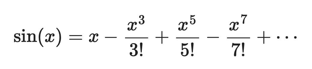
साइन फलन ऐसी श्रेणी देता है जिसमें केवल x की विषम घातें होती हैं, और चिन्ह क्रम से धन और ऋण में बदलते हैं।

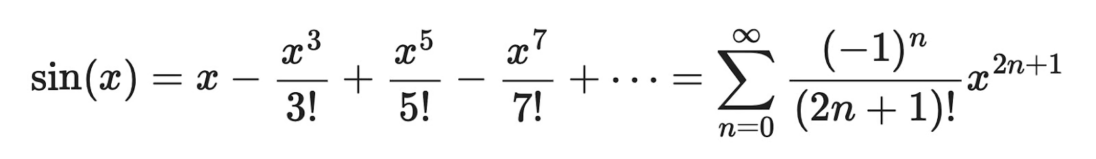
sin(x) का विस्तार

शून्य पर sin(x) के सम-क्रम के सभी अवकलज शून्य होते हैं, इसलिए वे पद गिर जाते हैं। बचता है विषम घातों का क्रम, हर के में फैक्टोरियल, और वैकल्पिक चिन्ह। eˣ की तरह, यह श्रेणी भी सभी x के लिए अभिसारी है।

cos(x)

कोसाइन का विस्तार साइन का प्रतिबिंब है — केवल x की सम घातें आती हैं, उसी वैकल्पिक चिन्ह पैटर्न के साथ।

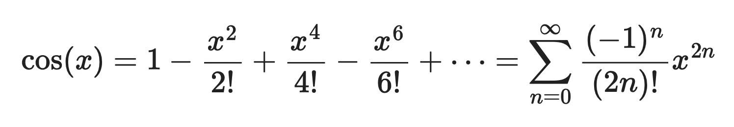
cos(x) का विस्तार

यह तर्कसंगत है क्योंकि cos(x), sin(x) का अवकलज है, और आप इस श्रेणी को sin(x) के विस्तार का पद-प्रतिपद अवकलन करके पा सकते हैं। विषम-घात वाले पद उसी कारण से गायब हो जाते हैं जिस कारण साइन में सम-घात वाले पद गायब हुए — शून्य पर अवकलज उन्हें शून्य कर देते हैं। यह भी सभी x के लिए अभिसारी है।

1 / (1 − x)

इन चार में यह सबसे सरल पैटर्न देता है: हर गुणांक बस 1 होता है, न कोई फैक्टोरियल, न वैकल्पिक चिन्ह।

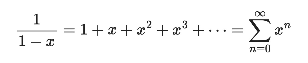
1/(1-x) का विस्तार

यह एक ज्यामितीय श्रेणी है, इसलिए पैटर्न इतना सुथरा दिखता है। लेकिन ऊपर के तीन फलनों के विपरीत, यह श्रेणी केवल तब अभिसरित होती है जब |x| < 1 हो। अगर आप x को उस दायरे के बाहर रखते हैं, तो पद शून्य की ओर सिमटने के बजाय अनियंत्रित रूप से बढ़ते हैं।

अंत में, दृश्य शिक्षार्थियों के लिए, यहाँ सभी चार श्रेणी-विस्तारों का बहुपद के कई पदों के साथ चार्ट तुलना है:

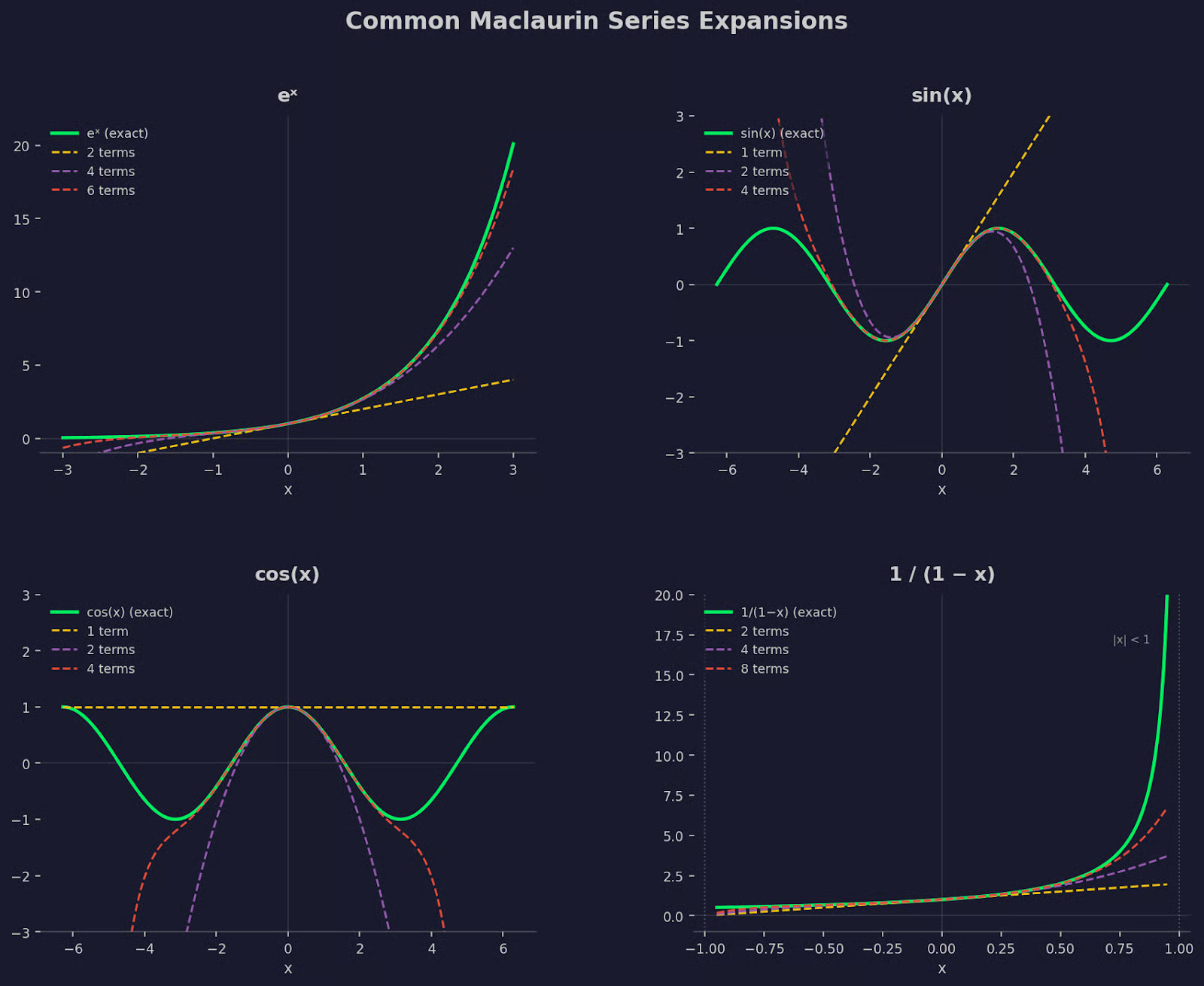
सामान्य मैक्लॉरिन श्रेणियाँ

मैक्लॉरिन श्रेणी से फलनों का सन्निकटन

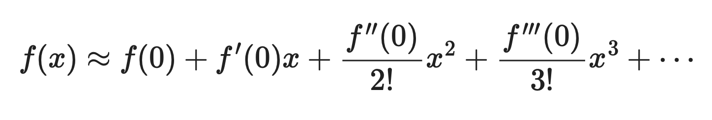
मैक्लॉरिन श्रेणी को उपयोगी होने के लिए शायद ही कभी उसके सभी अनंत पदों की जरूरत पड़ती है। व्यवहार में, आप आंशिक योग लेते हैं — शुरुआती कुछ पद — और उसे सन्निकटन के रूप में उपयोग करते हैं।

जितने अधिक पद शामिल करेंगे, आंशिक योग मूल फलन के उतना ही करीब चलेगा। यदि आप इसे दो पदों पर रोकते हैं, तो शून्य के पास एक मोटा-मोटा सन्निकटन मिलता है। कुछ और पद जोड़ने पर सन्निकटन और दूर तक मान्य रहता है। हर नया पद उन बातों को ठीक करता है जिन्हें पिछले पदों ने छोड़ा था।

sin(x) को एक ठोस उदाहरण मानें। पूरी श्रेणी यह है:

sin(x) सन्निकटन सूत्र

आइए sin(0.3) को आंशिक योगों से लगभगित करें और देखें कि हर एक सटीक मान से कैसे तुलना करता है।

• 1 पद: 0.3 — त्रुटि ~0.0045

• 2 पद: 0.3 - (0.3³/6) = 0.2955 — त्रुटि ~0.0000196

• 3 पद: जोड़ता है (0.3⁵/120) = 0.29552 — त्रुटि ~0.0000000239

तीन पद आपको छह दशमलव स्थानों तक की सटीकता दे देते हैं, जो पर्याप्त होनी चाहिए। अधिकांश मामलों में आपको इससे आगे जाने की ज़रूरत नहीं होती।

यही विचार Python में भी देखें:

import numpy as np
from math import factorial

def maclaurin_sin(x, n_terms):
    return sum(((-1)**n * x**(2*n+1)) / factorial(2*n+1) for n in range(n_terms))

vec_sin = np.vectorize(maclaurin_sin)
x_val = 0.3

print(f"Approximating sin({x_val}):")
print(f"  Exact value : {np.sin(x_val):.10f}")
for n in [1, 2, 3, 4]:
    approx = maclaurin_sin(x_val, n)
    error = abs(np.sin(x_val) - approx)
    print(f"  {n} term(s)   : {approx:.10f}  |  error: {error:.2e}"

इसे चलाने पर x = 0.3 पर आंशिक योगों के मान और त्रुटियाँ छपती हैं:

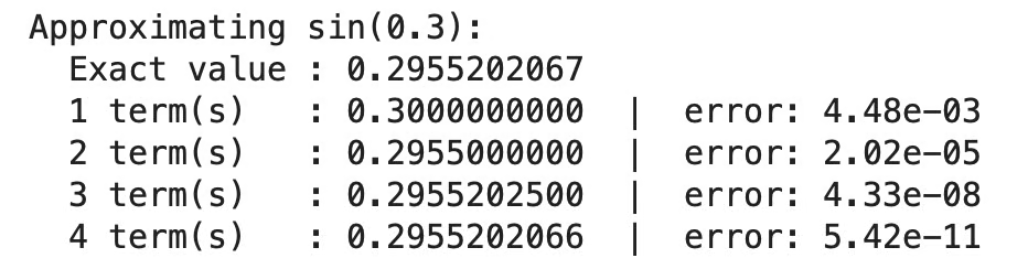
sin(x) के मैक्लॉरिन सन्निकटन का Python उदाहरण

इसे दृश्य रूप में भी परखा जा सकता है:

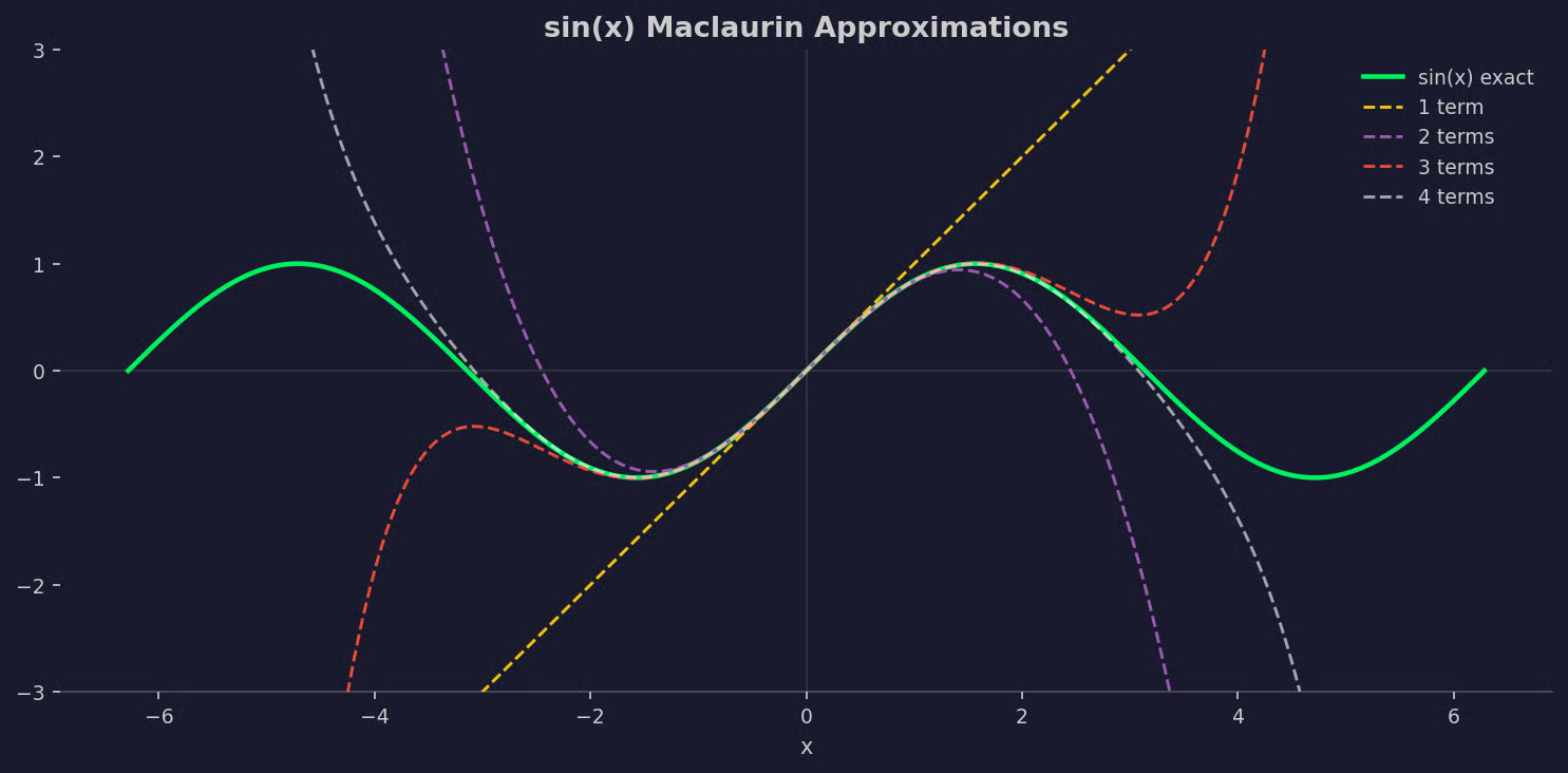
sin(x) मैक्लॉरिन सन्निकटन का चार्ट

आप देख सकते हैं कि प्रत्येक सन्निकटन sin(x) फलन को कितनी अच्छी तरह ट्रैक करता है।

मैक्लॉरिन श्रेणी का अभिसरण

मैक्लॉरिन श्रेणी हर x मान के लिए हमेशा काम नहीं करती। कुछ फलनों के लिए श्रेणी केवल शून्य के आसपास किसी विशेष दायरे में सही मान पर अभिसरित होती है। उस दायरे के बाहर, आंशिक योग घटने के बजाय अनियंत्रित रूप से बढ़ते हैं।

इस दायरे को अभिसरण त्रिज्या कहते हैं। यह बताती है कि शून्य से कितनी दूरी तक श्रेणी भरोसेमंद रहती है।

व्यवहार फलन पर निर्भर करता है:

• eˣ, sin(x), cos(x) — सभी x मानों के लिए अभिसरित होते हैं। आप कोई भी संख्या रखें और श्रेणी सही उत्तर देगी

• 1/(1-x) — केवल तब अभिसरित होती है जब |x| < 1 हो। x = 1 पर स्वयं फलन असीमित हो जाता है, और श्रेणी भी उसके पास अभिसरण करने में विफल रहती है

अभिसरण त्रिज्या को शून्य केंद्रित भरोसे के वृत्त की तरह सोचें। श्रेणी उसके अंदर ही मान्य सन्निकटन देती है।

हर बार अभिसरण त्रिज्या निकालना आवश्यक नहीं है। मानक फलनों के लिए यह ज्ञात होता है। लेकिन कम परिचित फलन पर काम करते समय, मैक्लॉरिन सन्निकटन पर निर्भर होने से पहले अभिसरण जाँचना अच्छी आदत है।

मैक्लॉरिन श्रेणी क्यों महत्वपूर्ण है

मैक्लॉरिन श्रेणियाँ गणना-आधारित कार्यों में, गणित, भौतिकी और मशीन लर्निंग में बार-बार आती हैं।

संख्यात्मक विधियाँ

कंप्यूटर अधिकांश फलनों का सांकेतिक मान नहीं निकालते। वे बहुपदों का मान निकालते हैं। जब कोई लाइब्रेरी sin(x) या eˣ की गणना करती है, तो वह अक्सर बहुपदीय सन्निकटन का उपयोग करती है — जो फलन के मैक्लॉरिन या टेलर विस्तार से निकला होता है। यह श्रेणी ऐसा रूप देती है जिसे हार्डवेयर तेज़ी से और बिना अनंत पुनरावृत्तियों के गणना कर सके।

भौतिकी में सन्निकटन

भौतिकी में जब सटीक हल के साथ काम करना बहुत जटिल हो, तब मैक्लॉरिन श्रेणी का उपयोग होता है। सबसे आम उदाहरण छोटा-कोण सन्निकटन है: छोटे θ के लिए, sin(θ) ≈ θ। यह sin(x) की मैक्लॉरिन श्रेणी का पहला ही पद है। यह लोलक समीकरणों, प्रकाशिकी गणनाओं और तरंग मॉडलों को सरल बनाता है — गैर-रैखिक समस्याओं को रैखिक में बदल कर जिन्हें वास्तव में हल किया जा सके।

मशीन लर्निंग और ऑप्टिमाइज़ेशन

मशीन लर्निंग में, टेलर और मैक्लॉरिन विस्तार उस गणित के पीछे हैं जिससे आप रोज़ रूबरू होते हैं। ग्रेडिएंट डिसेंट हानि फलन के प्रथम-क्रम सन्निकटन से तय करता है कि किस दिशा में कदम रखना है। न्यूटन विधि जैसे द्वितीय-क्रम तरीकों में वक्रता-पद का उपयोग होता है। जब शोधकर्ता किसी मॉडल के लॉस सरफेस के स्थानीय व्यवहार का विश्लेषण करते हैं, तो वे अक्सर किसी बिंदु के आसपास टेलर विस्तार की ही भाषा में सोचते हैं।

मैक्लॉरिन श्रेणी यही भी बताती है कि सैद्धांतिक विश्लेषण में sigmoid और tanh जैसे सक्रियण फलनों का सन्निकटन कैसे किया जाता है। उन्हें बहुपद के रूप में विस्तृत करने से ग्रेडिएंट और सेचुरेशन व्यवहार को समझना आसान हो जाता है।

निष्कर्ष

मैक्लॉरिन श्रेणी एक काम करती है: वह किसी फलन को शून्य पर केंद्रित बहुपद के रूप में लगभगित करती है। यह एक सरल विचार है जिसकी पहुँच बहुत दूर तक है।

संख्यात्मक कंप्यूटिंग से लेकर भौतिकी और मशीन लर्निंग तक, पैटर्न हमेशा एक जैसा है: किसी जटिल फलन को लें, उसे पर्याप्त नज़दीक आने वाले बहुपद से बदलें, और असली समस्या पर आगे बढ़ें। ग्रेडिएंट डिसेंट, छोटा-कोण सन्निकटन, और लाइब्रेरी के बिल्ट-इन फलनों के पीछे का गणित इसी मूल विचार तक जाता है।

eˣ, sin(x), cos(x), और 1/(1-x) के विस्तार याद रखने लायक हैं। ये इतने अक्सर आते हैं कि एक नज़र में पहचान लेना सचमुच समय बचाता है, खासकर जब आप शोध-पत्र पढ़ रहे हों।