Series de Maclaurin: fórmula, desarrollo y ejemplos

Algunas funciones son demasiado complejas para trabajar con ellas directamente, así que los matemáticos idearon cómo "fingirlas" con polinomios.

Esa es la idea básica detrás de una serie de Maclaurin. Representa una función como una suma infinita de términos polinómicos, cada uno construido a partir de las derivadas de la función en cero. El resultado es algo con lo que puedes calcular, incluso cuando la función original es demasiado compleja.

Puedes pensar en una serie de Maclaurin como un caso particular de la serie de Taylor, simplemente centrada en cero. Esa restricción la hace más sencilla de deducir y más fácil de aplicar.

En este artículo, veremos la fórmula de la serie de Maclaurin, repasaremos los desarrollos más comunes y te mostraré cómo interpretarlos y aplicarlos.

¿Qué es una serie de Maclaurin?

Una serie de Maclaurin representa una función como una suma infinita de términos construidos a partir de sus derivadas en cero.

Cada término es un polinomio: una potencia de x escalada por un valor de derivada. Al combinar suficientes términos, obtienes un polinomio que se comporta como la función original, al menos cerca de cero.

Aproximar una función compleja con un polinomio es la idea central de la serie de Maclaurin. Los polinomios son fáciles de calcular, derivar e integrar. La mayoría de las demás funciones no lo son.

Serie de Maclaurin vs. serie de Taylor

Una serie de Taylor aproxima una función como un polinomio infinito centrado en cualquier punto a. Eliges el punto, construyes la serie alrededor de él y obtienes un polinomio que funciona bien cerca de ese punto.

Una serie de Maclaurin es simplemente una serie de Taylor donde a = 0. Esa es la única diferencia.

Centrar en cero simplifica las cuentas porque los términos polinómicos eliminan el desplazamiento (x - a) y se convierten en potencias simples de x. La mayoría de funciones estándar con las que trabajarás en cálculo, física y machine learning tienen desarrollos de Maclaurin limpios y bien conocidos por este motivo.

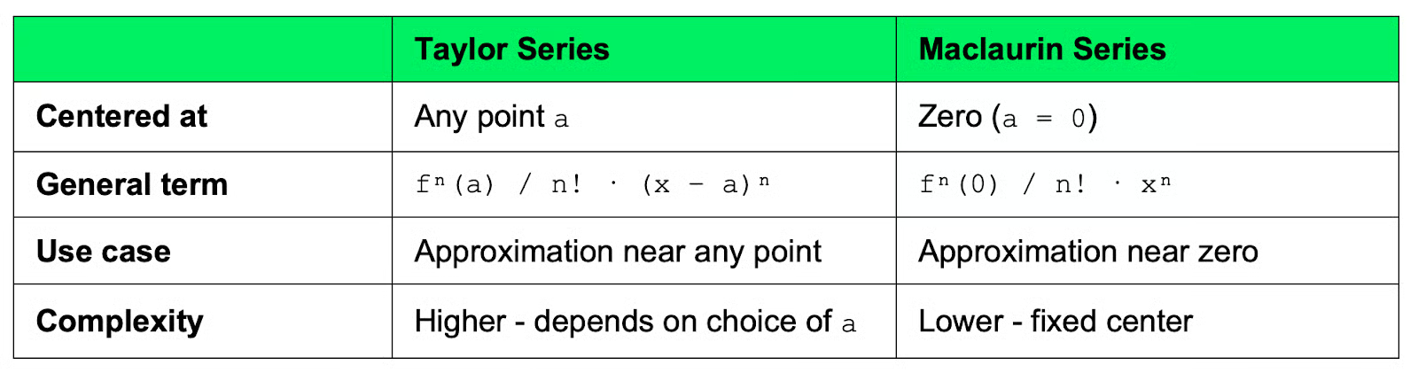
Comparación entre series de Taylor y Maclaurin

En resumen: usa una serie de Taylor cuando necesites aproximar una función cerca de un punto específico distinto de cero. Usa una serie de Maclaurin cuando cero sea el punto de partida, que suele serlo.

Fórmula de la serie de Maclaurin

La fórmula de la serie de Maclaurin expresa cualquier función f(x) como una suma infinita:

Fórmula de la serie de Maclaurin

Desarrollada, queda así:

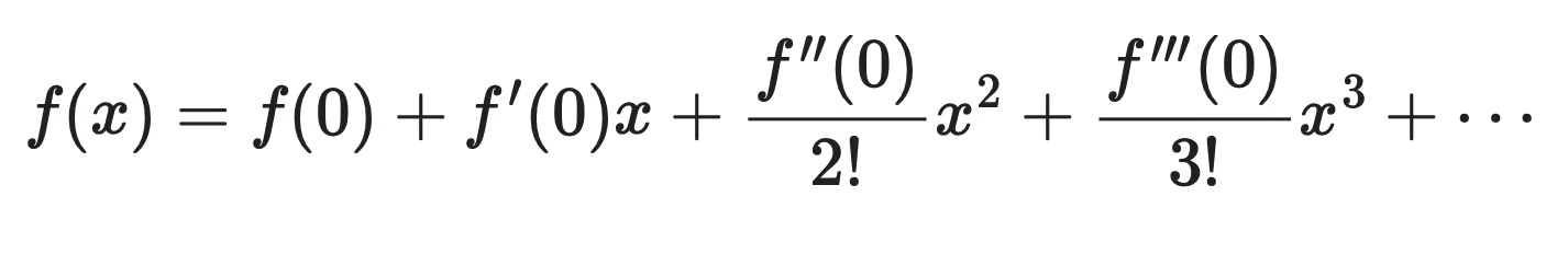
Fórmula de la serie de Maclaurin desarrollada

Cada término tiene tres partes:

• f⁽ⁿ⁾(0): la enésima derivada de f evaluada en cero. Indica cómo se comporta la función en ese punto

• n!: el factorial de n, que reduce cada término para que la serie se mantenga bien comportada a medida que crece n

• xⁿ: la enésima potencia de x, que determina hasta qué distancia de cero llega cada término

El primer término f(0) fija el valor del polinomio al de la función en cero. Cada término siguiente añade una corrección: ajusta la pendiente, la curvatura, etc., hasta que el polinomio se aproxime tanto como necesites a la función original.

En pocas palabras, cuantos más términos incluyas, mejor será la aproximación.

Cómo funciona la serie de Maclaurin

Construir una serie de Maclaurin se reduce a una acción repetida: evaluar derivadas en cero y apilar los resultados en un polinomio.

Así funciona, paso a paso.

1. Evalúa la función en cero: sustituye x = 0 en f(x). Esto te da el primer término: la constante que fija el valor inicial del polinomio
2. Toma las derivadas: calcula f'(x), f''(x), f'''(x), y así sucesivamente. En cada paso, evalúa el resultado en cero. Cada valor te cuenta algo sobre el comportamiento de la función: su pendiente, su curvatura, cómo cambia esa curvatura
3. Construye el polinomio: toma cada valor de derivada, divídelo por el factorial correspondiente y multiplícalo por la potencia de x que toque

Ahora suma todos los términos:

Cómo funciona la serie de Maclaurin

Cada término mejora la aproximación. El primero ajusta el valor. El segundo, la pendiente. El tercero, la curvatura. Y así sucesivamente.

Paras cuando la aproximación sea lo bastante buena para tu caso, o sigues si necesitas más precisión.

Desarrollos de Maclaurin más comunes

Hay funciones que aparecen tan a menudo que merece la pena memorizar sus desarrollos de Maclaurin. Aquí tienes las cuatro más habituales.

eˣ

La exponencial es el caso más sencillo: cada derivada de eˣ sigue siendo eˣ, lo que implica que todas las derivadas evaluadas en cero valen 1.

Desarrollo de e^x

Los coeficientes son simplemente 1/n!. La serie converge para todos los valores de x, lo que la convierte en uno de los desarrollos más útiles en la práctica.

sin(x)

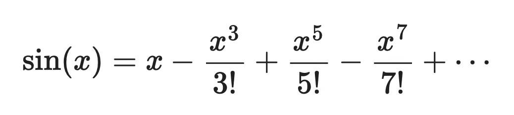
La función seno produce una serie con solo potencias impares de x, y los signos alternan entre positivos y negativos.

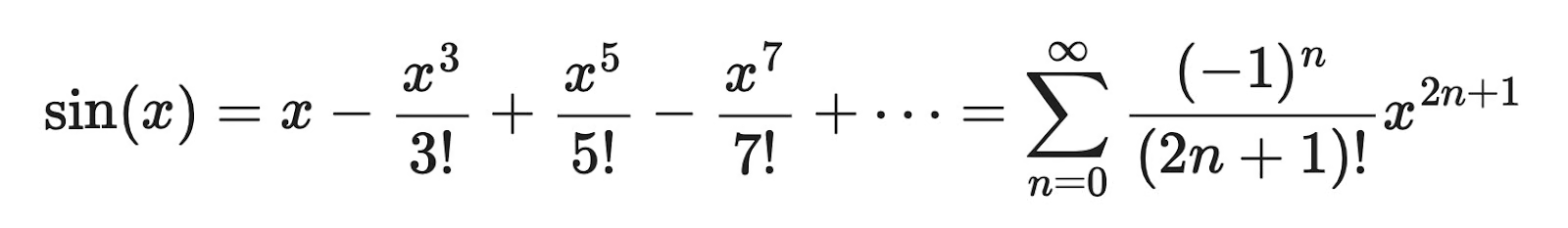
Desarrollo de sin(x)

Las derivadas de orden par de sin(x) en cero son todas nulas, así que esos términos desaparecen. Lo que queda son potencias impares, factoriales en el denominador y signos alternos. Al igual que eˣ, esta serie converge para todo x.

cos(x)

El desarrollo del coseno es la imagen especular del seno: solo aparecen potencias pares de x, con el mismo patrón de signos alternos.

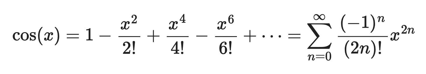
Desarrollo de cos(x)

Tiene sentido, ya que cos(x) es la derivada de sin(x), y puedes obtener esta serie derivando término a término el desarrollo de sin(x). Los términos con potencias impares desaparecen por la misma razón por la que en el seno desaparecen los pares: las derivadas en cero los anulan. Converge para todo x.

1 / (1 − x)

Este caso tiene el patrón más simple de los cuatro: todos los coeficientes valen 1, sin factoriales ni signos alternos.

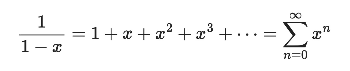
Desarrollo de 1/(1-x)

Es una serie geométrica, de ahí que el patrón sea tan limpio. Pero, a diferencia de las tres funciones anteriores, esta serie solo converge cuando |x| < 1. Si eliges x fuera de ese intervalo, los términos crecen sin límite en lugar de acercarse a cero.

Para quienes aprenden mejor con imágenes, aquí tienes una comparación gráfica de los cuatro desarrollos con varios términos:

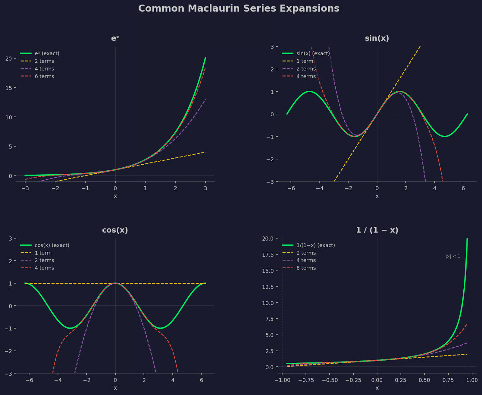
Series de Maclaurin comunes

Aproximar funciones con series de Maclaurin

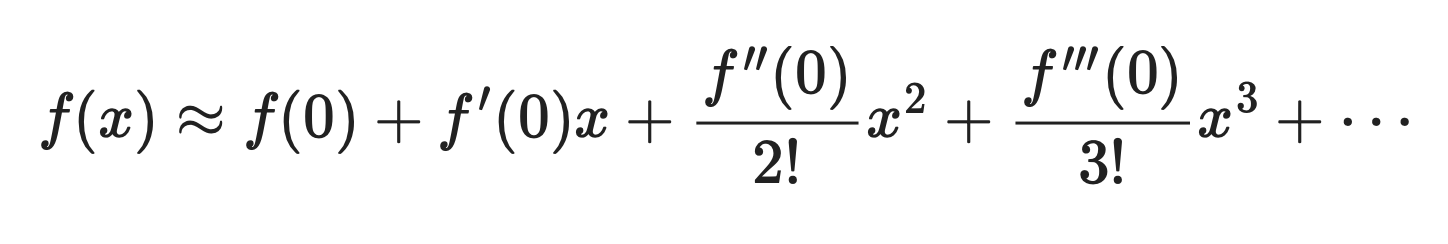
Rara vez necesitas todos los términos infinitos de una serie de Maclaurin para que sea útil. En la práctica, tomas una suma parcial (los primeros términos) y la usas como aproximación.

Cuantos más términos incluyas, mejor seguirá la suma parcial a la función original. Si cortas en dos términos, encaja de forma burda cerca de cero. Al añadir unos cuantos más, la aproximación aguanta más lejos. Cada término nuevo corrige lo que los anteriores no captaron.

Toma sin(x) como ejemplo concreto. La serie completa es:

Fórmula de aproximación de sin(x)

Vamos a aproximar sin(0.3) usando sumas parciales y ver cómo se compara cada una con el valor exacto.

• 1 término: 0.3 - error de ~0.0045

• 2 términos: 0.3 - (0.3³/6) = 0.2955 - error de ~0.0000196

• 3 términos: añade (0.3⁵/120) = 0.29552 - error de ~0.0000000239

Con tres términos alcanzas precisión de seis decimales, más que suficiente en la mayoría de los casos. Normalmente no hace falta ir mucho más allá.

La misma idea en Python:

import numpy as np
from math import factorial

def maclaurin_sin(x, n_terms):
    return sum(((-1)**n * x**(2*n+1)) / factorial(2*n+1) for n in range(n_terms))

vec_sin = np.vectorize(maclaurin_sin)
x_val = 0.3

print(f"Approximating sin({x_val}):")
print(f"  Exact value : {np.sin(x_val):.10f}")
for n in [1, 2, 3, 4]:
    approx = maclaurin_sin(x_val, n)
    error = abs(np.sin(x_val) - approx)
    print(f"  {n} term(s)   : {approx:.10f}  |  error: {error:.2e}"

Al ejecutar esto, se imprimen los valores de las sumas parciales y los errores en x = 0.3:

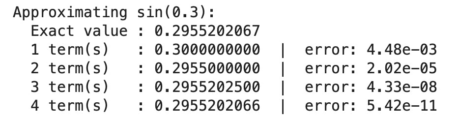
Ejemplo en Python de la aproximación de Maclaurin de sin(x)

También puedes verlo de forma visual:

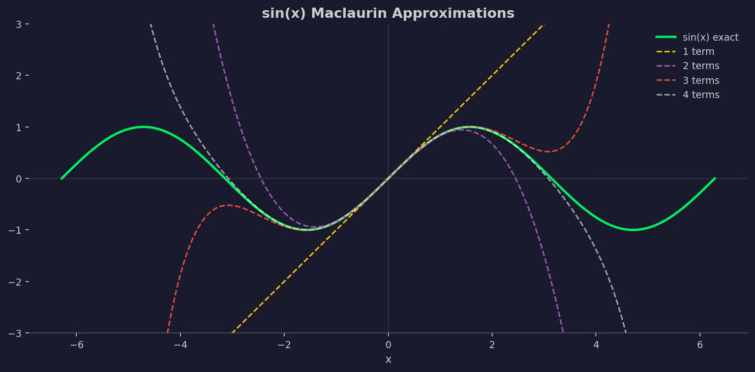
Gráfico de la aproximación de Maclaurin de sin(x)

Puedes ver lo bien que sigue cada aproximación a la función sin(x).

Convergencia de las series de Maclaurin

Una serie de Maclaurin no siempre funciona para cualquier valor de x. En algunas funciones, la serie converge al valor correcto solo dentro de un rango específico alrededor de cero. Fuera de ese rango, las sumas parciales crecen sin límite.

A este rango se le llama radio de convergencia. Indica hasta qué distancia de cero la serie sigue siendo fiable.

El comportamiento varía según la función:

• eˣ, sin(x), cos(x): convergen para todos los valores de x. Puedes introducir cualquier número y la serie te dará el resultado correcto

• 1/(1-x): solo converge cuando |x| < 1. En x = 1 la propia función se dispara, y la serie lo refleja al no converger cerca de ese punto

Piensa en el radio de convergencia como un círculo de confianza centrado en cero. La serie es una aproximación válida solo dentro de él.

No siempre necesitas calcular el radio de convergencia. En las funciones estándar, es un dato conocido. Pero si trabajas con una función menos familiar, comprobar la convergencia antes de fiarte de una aproximación de Maclaurin es una buena práctica.

Por qué importan las series de Maclaurin

Las series de Maclaurin aparecen en trabajos computacionales reales en matemáticas, física y machine learning.

Métodos numéricos

Los ordenadores no pueden evaluar la mayoría de funciones de forma simbólica. Evalúan polinomios. Cuando una librería calcula sin(x) o eˣ, a menudo usa una aproximación polinómica derivada del desarrollo de Maclaurin o Taylor. La serie te da una forma que el hardware puede calcular de verdad, rápido y sin bucles infinitos.

Aproximaciones en física

La física recurre a series de Maclaurin siempre que una solución exacta es demasiado compleja. El ejemplo más común es la aproximación para ángulos pequeños: para valores pequeños de θ, sin(θ) ≈ θ. Es solo el primer término de la serie de Maclaurin de sin(x). Simplifica ecuaciones de péndulos, cálculos de óptica y modelos de ondas, convirtiendo problemas no lineales en lineales que sí se pueden resolver.

Machine learning y optimización

En machine learning, los desarrollos de Taylor y Maclaurin están detrás de gran parte de las matemáticas del día a día. El descenso por gradiente usa aproximaciones de primer orden de la función de pérdida para decidir hacia dónde avanzar. Los métodos de segundo orden, como el de Newton, usan el término de curvatura. Cuando se analiza localmente la superficie de pérdida de un modelo, a menudo se piensa en términos de desarrollos de Taylor alrededor de un punto.

La serie de Maclaurin también se usa para aproximar, en análisis teórico, funciones de activación como sigmoid y tanh. Desarrollarlas en polinomios facilita razonar sobre gradientes y saturación.

Conclusión

Una serie de Maclaurin hace una cosa: aproxima una función con un polinomio centrado en cero. Es una idea simple con un alcance enorme.

Desde el cálculo numérico hasta la física y el machine learning, el patrón se repite: toma una función compleja, sustitúyela por un polinomio lo bastante cercano y céntrate en el problema real. Las matemáticas detrás del descenso por gradiente, las aproximaciones de ángulo pequeño y muchas funciones de librería parten de esta misma idea.

Los desarrollos de eˣ, sin(x), cos(x) y 1/(1-x) merecen la pena memorizarlos. Aparecen con tanta frecuencia que reconocerlos al vuelo ahorra tiempo, sobre todo si lees artículos de investigación.