Contingency Analysis using R

Contingency analysis is a hypothesis test that is used to check whether two categorical variables are independent or not. In simple words, we are asking the question "Can we predict the value of one variable if we know the value of the other variable?". If the answer is yes, we can say that the variables under consideration are not independent. If the answer is no, then we can say that the variables under consideration are independent. The test makes use of contingency tables as a result of which it is known as 'Contingency Analysis'. It is also known as 'Chi-square test of independence' because the test statistic follows a chi-square distribution and the test is used to check whether two categorical variables are independent or not.

The null hypothesis of the test is that the two variables are independent and the alternative hypothesis is that the two variables are not independent.

Let us try to understand 'Contingency Analysis' or 'Chi-square test of independence' with the help of an example.

Suppose we want to know whether the choice of sport is independent of gender or not. So, we asked one hundred men and one hundred women which sport they prefer to play among archery, boxing, and cycling and summarizes the data obtained in the following two-way table.

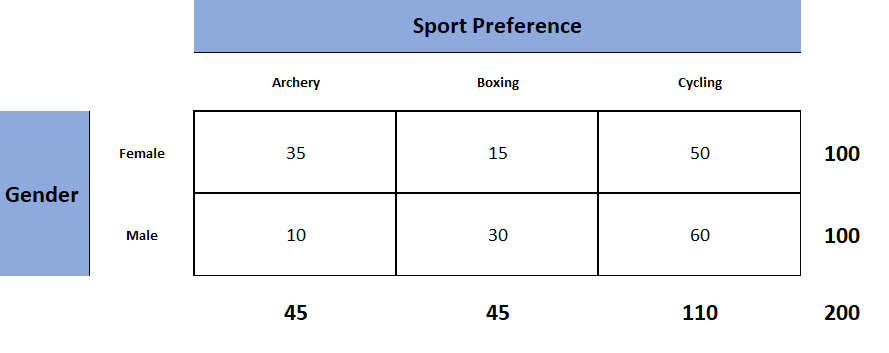
The above table is known as the observed table as it contains the observed counts.

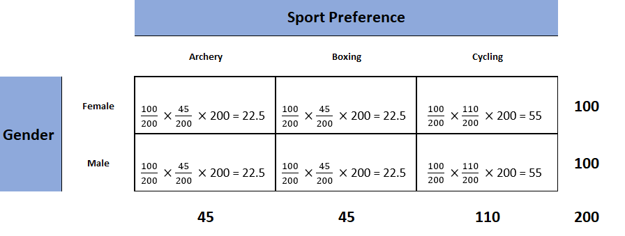
The Chi-square test of independence works by comparing the observed counts to the expected counts. Therefore, our next task is to derive the expected table containing the expected counts from the observed table. The expected table is what we expect the two-way table to look like if the two categorical variables are independent. From probability theory, we know that two events are said to be independent if their joint probability is equal to the product of their marginal probabilities. We will use this concept to calculate the expected counts for each of the six cells. Let us compute the expected count for the first cell. First, we will calculate the joint probability by multiplying the probability of being female (100/200) with the probability of preferring archery (45/200). Once we have the joint probability (100/200 * 45/200), if we multiply it by the sample size (200) we will get the expected count for the first cell which is 22.5. Similarly, we will compute the expected counts for the remaining five cells. The following table is the table that we want to see if gender and sports preference are independent.

Now that we have the expected as well as the observed counts, our next task is to check how different the observed counts are from the expected counts. For that purpose, we have to compute a test statistic known as the chi-square test static as it follows the chi-square distribution. Following is the formula for computing the value of the chi-square test statistic.

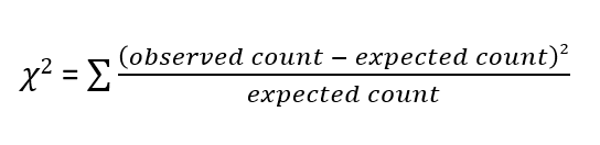
We can see from the above formula that the value of the chi-square test statistic can be 0 (when there is absolutely no difference between the observed and the expected counts) but can never be negative. This makes the Chi-square test of independence a one-tailed test.

Using the above formula let us calculate the value of the chi-square test statistic for our example. It is known as the observed value of the test statistic.

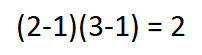
Now it is time to decide whether to reject the null hypothesis or not. We make the decision either by comparing the observed value of the test statistic to its critical value or by looking at the p-value. If the observed value of the test statistic exceeds its critical value or if the p-value is less than or equal to the significance level then we can reject the null hypothesis and conclude that there is a statistically significant relationship between the two categorical variables that is they are not independent. If we know the significance level (usually 0.05) and the degrees of freedom we can get the critical value from the chi-square table. The significance level is the probability of rejecting a true null hypothesis. For a table with r rows and c columns, degrees of freedom can be calculated by the following formula.

Therefore, for our example, we have 2 degrees of freedom.

From the below table we can see that the critical value of the test statistic is 5.99 for a significance level of 0.05 and 2 degrees of freedom.

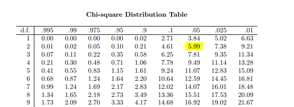
Since the observed value of the test statistic is greater than its critical value (19.798 > 5.99), we can reject the null hypothesis and conclude that choice of sport is not independent of gender.

Let us now see how to perform the Chi-square test of independence using R programming language

It is very easy to perform the Chi-square test of independence using the built-in function chisq.test().

Following is the observed table.

observed_table <- matrix(c(35, 15, 50, 10, 30, 60), nrow = 2, ncol = 3, byrow = T)
rownames(observed_table) <- c('Female', 'Male')
colnames(observed_table) <- c('Archery', 'Boxing', 'Cycling')
observed_table

##        Archery Boxing Cycling
## Female      35     15      50
## Male        10     30      60

In order to perform the test, we need to apply the chisq.test() function to the observed table.

X <- chisq.test(observed_table)
X

##
##  Pearson's Chi-squared test
##
## data:  observed_table
## X-squared = 19.798, df = 2, p-value = 5.023e-05

From the above result, we can see that p-value is less than the significance level (0.05). Therefore, we can reject the null hypothesis and conclude that the two variables (gender & sport preference) are not independent.

If we want to see the expected table, we can also do that.

X$expected

##        Archery Boxing Cycling
## Female    22.5   22.5      55
## Male      22.5   22.5      55

I hope you enjoyed this article. If you would like to learn more in R, take DataCamp's Statistical Modeling in R (Part 1) course.