Course
Technology has become an asset in finance: financial institutions are now evolving to technology companies rather than only staying occupied with just the financial aspect: besides the fact that technology brings about innovation the speeds and can help to gain a competitive advantage, the rate and frequency of financial transactions, together with the large data volumes, makes that financial institutions' attention for technology has increased over the years and that technology has indeed become the main enabler in finance.
Among the hottest programming languages for finance, you'll find R and Python, alongside languages such as C++, C#, and Java. In this tutorial, you'll learn how to get started with Python for finance. The tutorial will cover the following:
Download the Jupyter notebook of this tutorial here.
Getting Started with Python for Finance
Before you go into trading strategies, it's a good idea to get the hang of the basics first. This first part of the tutorial will focus on explaining the Python basics that you need to get started. This does not mean, however, that you'll start entirely from zero: you should have at least done DataCamp's free Intro to Python for Data Science course, in which you learned how to work with Python lists, packages, and NumPy. Additionally, it is desired to already know the basics of Pandas, the popular Python data manipulation package, but this is no requirement.
Then I would suggest you take DataCamp's Intro to Python for Finance course to learn the basics of finance in Python. If you then want to apply your new 'Python for Data Science' skills to real-world financial data, consider taking the Importing and Managing Financial Data in Python course.
Stocks & Trading
When a company wants to grow and undertake new projects or expand, it can issue stocks to raise capital. A stock represents a share in the ownership of a company and is issued in return for money. Stocks are bought and sold: buyers and sellers trade existing, previously issued shares. The price at which stocks are sold can move independent of the company's success: the prices instead reflect supply and demand. This means that whenever a stock is considered as ‘desirable', due to success, popularity, … the stock price will go up.
Note that stocks are not the same as bonds, which is when companies raise money through borrowing, either as a loan from a bank or by issuing debt.
As you just read, buying and selling or trading is essential when you're talking about stocks, but certainly not limited to it: trading is the act of buying or selling an asset, which could be financial security, like stock, a bond or a tangible product, such as gold or oil.
Stock trading is then the process of the cash that is paid for the stocks is converted into a share in the ownership of a company, which can be converted back to cash by selling, and this all hopefully with a profit. Now, to achieve a profitable return, you either go long or short in markets: you either by shares thinking that the stock price will go up to sell at a higher price in the future, or you sell your stock, expecting that you can buy it back at a lower price and realize a profit. When you follow a fixed plan to go long or short in markets, you have a trading strategy.
Developing a trading strategy is something that goes through a couple of phases, just like when you, for example, build machine learning models: you formulate a strategy and specify it in a form that you can test on your computer, you do some preliminary testing or backtesting, you optimize your strategy and lastly, you evaluate the performance and robustness of your strategy.
Trading strategies are usually verified by backtesting: you reconstruct, with historical data, trades that would have occurred in the past using the rules that are defined with the strategy that you have developed. This way, you can get an idea of the effectiveness of your strategy, and you can use it as a starting point to optimize and improve your strategy before applying it to real markets. Of course, this all relies heavily on the underlying theory or belief that any strategy that has worked out well in the past will likely also work out well in the future, and, that any strategy that has performed poorly in the past will probably also do badly in the future.
Time Series Data
A time series is a sequence of numerical data points taken at successive equally spaced points in time. In investing, a time series tracks the movement of the chosen data points, such as the stock price, over a specified period of time with data points recorded at regular intervals. If you're still in doubt about what this would exactly look like, take a look at the following example:
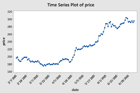
You see that the dates are placed on the x-axis, while the price is featured on the y-axis. The “successive equally spaced points in time” in this case means that the days that are featured on the x-axis are 14 days apart: note the difference between 3/7/2005 and the next point, 3/31/2005, and 4/5/2005 and 4/19/2005.
However, what you'll often see when you're working with stock data is not just two columns, that contain period and price observations, but most of the times, you'll have five columns that contain observations of the period and the opening, high, low and closing prices of that period. This means that, if your period is set at a daily level, the observations for that day will give you an idea of the opening and closing price for that day and the extreme high and low price movement for a particular stock during that day.
For now, you have a basic idea of the basic concepts that you need to know to go through this tutorial. These concepts will come back soon enough, and you'll learn more about them later on in this tutorial.
Setting up the Workspace
Getting your workspace ready to go is an easy job: just make sure you have Python and an Integrated Development Environment (IDE) running on your system. However, there are some ways in which you can get started that are maybe a little easier when you're just starting out.
Take for instance Anaconda, a high-performance distribution of Python and R and includes over 100 of the most popular Python, R and Scala packages for data science. Additionally, installing Anaconda will give you access to over 720 packages that can easily be installed with conda, our renowned package, dependency and environment manager, that is included in Anaconda. And, besides all that, you'll get the Jupyter Notebook and Spyder IDE with it.
That sounds like a good deal, right?
You can install Anaconda from here and don't forget to check out how to set up your Jupyter Notebook in DataCamp's Jupyter Notebook Tutorial: The Definitive Guide.
Of course, Anaconda is not your only option: you can also check out the Canopy Python distribution (which doesn't come free), or try out the Quant Platform.
The latter offers you a couple of additional advantages over using, for example, Jupyter or the Spyder IDE, since it provides you everything you need specifically to do financial analytics in your browser! With the Quant Platform, you'll gain access to GUI-based Financial Engineering, interactive and Python-based financial analytics and your own Python-based analytics library. What's more, you'll also have access to a forum where you can discuss solutions or questions with peers!
Python Basics for Finance: Pandas
When you're using Python for finance, you'll often find yourself using the data manipulation package, Pandas. But also other packages such as NumPy, SciPy, Matplotlib,… will pass by once you start digging deeper.
For now, let's focus on Pandas and using it to analyze time series data. This section will explain how you can import data, explore and manipulate it with Pandas. On top of all of that, you'll learn how you can perform common financial analyses on the data that you imported.
Importing Financial Data into Python
The pandas-datareader package allows for reading in data from sources such as Google, World Bank,… If you want to have an updated list of the data sources that are made available with this function, go to the documentation. You used to be able to access data from Yahoo! Finance directly, but it has since been deprecated. To access Yahoo! Finance data, check out this video by Matt Macarty that shows a workaround. For this tutorial, you will use the package to read in data from Yahoo! Finance. Make sure to install the package first by installing the latest release version via pip with pip install pandas-datareader.
Tip: if you want to install the latest development version or if you experience any issues, you can read up on the installation instructions here.
import pandas_datareader as pdr
import datetime
aapl = pdr.get_data_yahoo('AAPL',
                          start=datetime.datetime(2006, 10, 1),
                          end=datetime.datetime(2012, 1, 1))
Run and edit the code from this tutorial online
Run codeNote that the Yahoo API endpoint has recently changed and that, if you want to already start working with the library on your own, you'll need to install a temporary fix until the patch has been merged into the master branch to start pulling in data from Yahoo! Finance with pandas-datareader. Make sure to read up on the issue here before you start on your own!
No worries, though, for this tutorial, the data has been loaded in for you so that you don't face any issues while learning about finance in Python with Pandas.
It's wise to consider though that, even though pandas-datareader offers a lot of options to pull in data into Python, it isn't the only package that you can use to pull in financial data: you can also make use of libraries such as Quandl, for example, to get data from Google Finance:
import quandl
aapl = quandl.get("WIKI/AAPL", start_date="2006-10-01", end_date="2012-01-01")
For more information on how you can use Quandl to get financial data directly into Python, go to this page.
Lastly, if you've already been working in finance for a while, you'll probably know that you most often use Excel also to manipulate your data. In such cases, you should know that you can integrate Python with Excel.
Check out DataCamp's Python Excel Tutorial: The Definitive Guide for more information.
Working with Time Series Data
The first thing that you want to do when you finally have the data in your workspace is getting your hands dirty. However, now that you're working with time series data, this might not seem as straightforward, since your index now contains DateTime values.
No worries, though! Let's start step-by-step and explore the data first with some functions that you might already know if you have some prior programming experience with R or if you've previously worked with Pandas.
Either way, you'll see it's pretty straightforward!
As you saw in the code chunk above, you have used pandas_datareader to import data into your workspace. The resulting object aapl is a DataFrame, which is a 2-dimensional labeled data structure with columns of potentially different types. Now, one of the first things that you probably do when you have a regular DataFrame on your hands, is running the head() and tail() functions to take a peek at the first and the last rows of your DataFrame. Luckily, this doesn't change when you're working with time series data!
Tip: also make sure to use the describe() function to get some useful summary statistics about your data.
Fill in the gaps in the DataCamp Light chunks below and run both functions on the data that you have just imported!
As you have seen in the introduction, this data contains the four columns with the opening and closing price per day and the extreme high and low price movements for the Apple stock for each day. Additionally, you also get two extra columns: Volume and Adj Close.
The former column is used to register the number of shares that got traded during a single day. The latter, on the other hand, is the adjusted closing price: it's the closing price of the day that has been slightly adapted to include any actions that occurred at any time before the next day's open. You can use this column to examine historical returns or when you're performing a detailed analysis on historical returns.
Note how the index or row labels contain dates, and how your columns or column labels contain numerical values.
Tip: if you now would like to save this data to a csv file with the to_csv() function from pandas and that you can use the read_csv() function to read the data back into Python. This is extremely handy in cases where, for example, the Yahoo API endpoint has changed, and you don't have access to your data any longer :)
import pandas as pd
aapl.to_csv('data/aapl_ohlc.csv')
df = pd.read_csv('data/aapl_ohlc.csv', header=0, index_col='Date', parse_dates=True)
Now that you have briefly inspected the first lines of your data and have taken a look at some summary statistics, it's time to go a little bit deeper.
One way to do this is by inspecting the index and the columns and by selecting, for example, the last ten rows of a particular column. The latter is called subsetting because you take a small subset of your data. The result of the subsetting is a Series, which is a one-dimensional labeled array that is capable of holding any type.
Remember that the DataFrame structure was a two-dimensional labeled array with columns that potentially hold different types of data.
Check all of this out in the exercise below. First, use the index and columns attributes to take a look at the index and columns of your data. Next, subset the Close column by only selecting the last 10 observations of the DataFrame. Make use of the square brackets [] to isolate the last ten values. You might already know this way of subsetting from other programming languages, such as R. To conclude, assign the latter to a variable ts and then check what type ts is by using the type() function:
The square brackets can be helpful to subset your data, but they are maybe not the most idiomatic way to do things with Pandas. That's why you should also take a look at the loc() and iloc() functions: you use the former for label-based indexing and the latter for positional indexing.
In practice, this means that you can pass the label of the row labels, such as 2007 and 2006-11-01, to the loc() function, while you pass integers such as 22 and 43 to the iloc() function.
Complete the exercise below to understand how both loc() and iloc() work:
Tip: if you look closely at the results of the subsetting, you'll notice that there are certain days missing in the data; If you look more closely at the pattern, you'll see that it's usually two or three days that are missing; These days are traditionally weekend days or public holidays and aren't part of your data. This is nothing to worry about: it's completely normal, and you don't have to fill in these missing days.
Besides indexing, you might also want to explore some other techniques to get to know your data a little bit better. You never know what else will show up. Let's try to sample some 20 rows from the data set and then let's resample the data so that aapl is now at the monthly level instead of daily. You can make use of the sample() and resample() functions to do this:
Very straightforward, isn't it?
The resample() function is often used because it provides elaborate control and more flexibility on the frequency conversion of your times series: besides specifying new time intervals yourself and specifying how you want to handle missing data, you also have the option to indicate how you want to resample your data, as you can see in the code example above. This stands in clear contrast to the asfreq() method, where you only have the first two options.
Tip: try this out for yourself in the IPython console of the above DataCamp Light chunk. Pass in aapl.asfreq("M", method="bfill") to see what happens!
Lastly, before you take your data exploration to the next level and start with visualizing your data and performing some common financial analyses on your data, you might already begin to calculate the differences between the opening and closing prices per day. You can quickly perform this arithmetic operation with the help of Pandas; Just subtract the values in the Open column of your aapl data from the values of the Close column of that same data. Or, in other words, deduct aapl.Close from aapl.Open. You store the result in a new column of the aapl DataFrame called diff, and then you delete it again with the help of del:
Tip: make sure to comment out the last line of code so that the new column of your aapl DataFrame doesn't get removed and you can check the results of your arithmetic operation!
Of course, knowing the gains in absolute terms might already help you to get an idea of whether you're making a good investment, but as a quant, you might be more interested in a more relative means of measuring your stock's value, like how much the value of a particular stock has gone up or gone down. A way to do this is by calculating the daily percentage change.
This is good to know for now, but don't worry about it just yet; You'll go deeper into this in a bit!
This section introduced you to some ways to first explore your data before you start performing some prior analyses. However, you can still go a lot further in this; Consider taking our Python Exploratory Data Analysis if you want to know more.
Visualizing Time Series Data
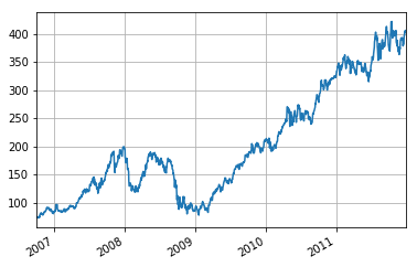
Next to exploring your data by means of head(), tail(), indexing, … You might also want to visualize your time series data. Thanks to Pandas' plotting integration with Matplotlib, this task becomes easy; Just use the plot() function and pass the relevant arguments to it. Additionally, you can also add the grid argument to indicate that the plot should also have a grid in the background.
Let's examine and run the code below to see how you can make this plot!
If you want to know more about Matplotlib and how to get started with it, check out DataCamp's Intermediate Python for Data Science course.
Common Financial Analysis
Now that you have an idea of your data, what time series data is about and how you can use pandas to explore your data quickly, it's time to dive deeper into some of the common financial analyses that you can do so that you can actually start working towards developing a trading strategy.
In the rest of this section, you'll learn more about the returns, moving windows, volatility calculation and Ordinary Least-Squares Regression (OLS).
Returns
The simple daily percentage change doesn't take into account dividends and other factors and represents the amount of percentage change in the value of a stock over a single day of trading. You will find that the daily percentage change is easily calculated, as there is a pct_change() function included in the Pandas package to make your life easier:
Note that you calculate the log returns to get a better insight into the growth of your returns over time.
Knowing how to calculate the daily percentage change is nice, but what when you want to know the monthly or quarterly returns? In such cases, you can fall back on the resample(), which you already saw in the first part of this tutorial.
Using pct_change() is quite the convenience, but it also obscures how exactly the daily percentages are calculated. That's why you can alternatively make use of Pandas' shift() function instead of using pct_change(). You then divide the daily_close values by the daily_close.shift(1) -1. By using this function, however, you will be left with NA values at the beginning of the resulting DataFrame.
Tip: compare the result of the following code with the result that you had obtained in the first DataCamp Light chunk to clearly see the difference between these two methods of calculating the daily percentage change.
Tip: calculate the daily log returns with the help of Pandas' shift() function. Try it out in the IPython console of this DataCamp Light chunk! (For those who can't find the solution, try out this line of code: daily_log_returns_shift = np.log(daily_close / daily_close.shift(1))).
For your reference, the calculation of the daily percentage change is based on the following formula: \(r_t = \dfrac{{p_t}}{p_{t-1}} - 1\), where p is the price, t is the time (a day in this case) and r is the return.
Additionally, you can plot the distribution of daily_pct_change:
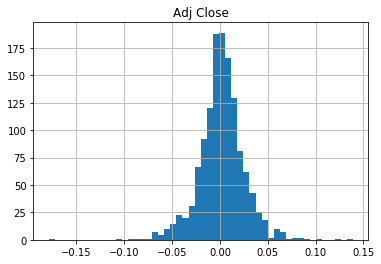
The distribution looks very symmetrical and normally distributed: the daily changes center around the bin 0.00. Note, though, how you can and should use the results of the describe() function, applied on daily_pct_c, to correctly interpret the results of the histogram. You will see that the mean is very close to the 0.00 bin also and that the standard deviation is 0.02. Also, take a look at the percentiles to know how many of your data points fall below -0.010672, 0.001677 and 0.014306.
The cumulative daily rate of return is useful to determine the value of an investment at regular intervals. You can calculate the cumulative daily rate of return by using the daily percentage change values, adding 1 to them and calculating the cumulative product with the resulting values:
Note that you can use can again use Matplotlib to quickly plot the cum_daily_return; Just add the plot() function to it and, optionally, determine the figsize or the size of the figure:
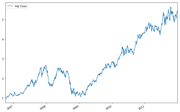
Very easy, isn't it? Now, if you don't want to see the daily returns, but rather the monthly returns, remember that you can easily use the resample() function to bring the cum_daily_return to the monthly level:
Knowing how to calculate the returns is a valuable skill, but you'll often see that these numbers don't really say much when you don't compare them to other stock. That's why you'll often see examples where two or more stocks are compared. In the rest of this section, you'll focus on getting more data from Yahoo! Finance so that you can calculate the daily percentage change and compare the results.
Note that, if you want to be doing this, you'll need to have a more thorough understanding of Pandas and how you can manipulate your data with Pandas!
Let's start! Get more data from Yahoo! Finance first. You can easily do this by making a function that takes in the ticker or symbol of the stock, a start date and an end date. The next function that you see, data(), then takes the ticker to get your data from the startdate to the enddate and returns it so that the get() function can continue. You map the data with the right tickers and return a DataFrame that concatenates the mapped data with tickers.
Check out the code below, where the stock data from Apple, Microsoft, IBM, and Google are loaded and gathered into one big DataFrame:
def get(tickers, startdate, enddate):
  def data(ticker):
    return (pdr.get_data_yahoo(ticker, start=startdate, end=enddate))
  datas = map (data, tickers)
  return(pd.concat(datas, keys=tickers, names=['Ticker', 'Date']))

tickers = ['AAPL', 'MSFT', 'IBM', 'GOOG']
all_data = get(tickers, datetime.datetime(2006, 10, 1), datetime.datetime(2012, 1, 1))
Note that this code originally was used in “Mastering Pandas for Finance”. It was updated for this tutorial to the new standards. Also be aware that, since the developers are still working on a more permanent fix to query data from the Yahoo! Finance API, it could be that you need to import the fix_yahoo_finance package. You can find the installation instructions here or check out the Jupyter notebook that goes along with this tutorial.
For the rest of this tutorial, you're safe, as the data has been loaded in for you!
Now, the result of these lines of code, you ask? Check it out:
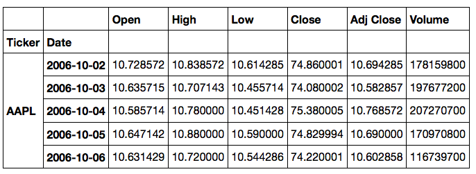
You can then use the big DataFrame to start making some interesting plots:
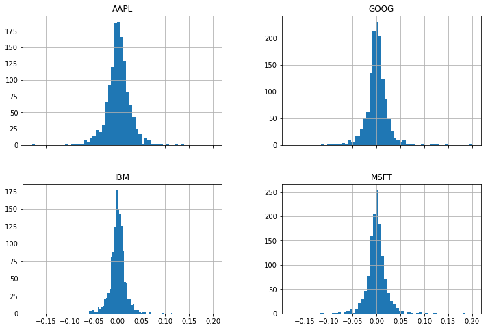
Another useful plot is the scatter matrix. You can easily do this by using the pandas library. Don't forget to add the scatter_matrix() function to your code so that you actually make a scatter matrix :) As arguments, you pass the daily_pct_change and as a diagonal, you set that you want to have a Kernel Density Estimate (KDE) plot. Additionally, you can set the transparency with the alpha argument and the figure size with figsize.
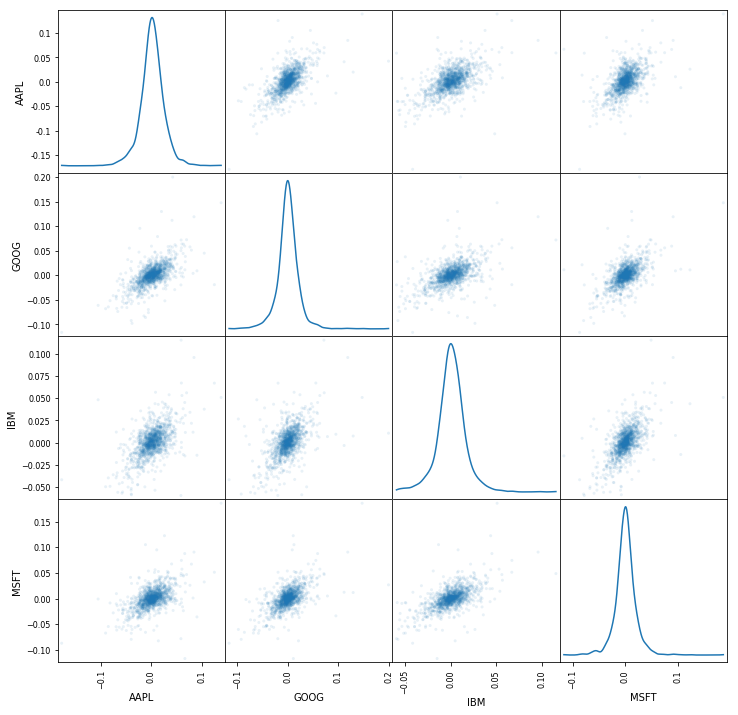
Note that you might need to use the plotting module to make the scatter matrix (i.e. pd.plotting.scatter_matrix()) when you're working locally. Also, it's good to know that the Kernel Density Estimate plot estimates the probability density function of a random variable.
Congratulations! You've successfully made it through the first common financial analysis, where you explored returns! Now it's time to move on to the second one, which are the moving windows.
Moving Windows
Moving windows are there when you compute the statistic on a window of data represented by a particular period of time and then slide the window across the data by a specified interval. That way, the statistic is continually calculated as long as the window falls first within the dates of the time series.
There are a lot of functions in Pandas to calculate moving windows, such as rolling_mean(), rolling_std(), … See all of them here.
However, note that most of them will soon be deprecated, so it's best to use a combination of the functions rolling() with mean() or std(),… Depending of course on which type of moving window you want to calculate exactly.
But what does a moving window exactly mean for you?
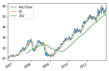
The exact meaning, of course, depends on the statistic that you're applying to the data. For example, a rolling mean smoothes out short-term fluctuations and highlight longer-term trends in data.
Tip: try out some of the other standard moving windows functions that come with the Pandas package, such as rolling_max(), rolling_var() or rolling_median(), in the IPython console. Note that you can also use rolling() in combination with max(), var() or median() to accomplish the same results! Remember that you can find more functions if you click on the link that's provided in the text on top of this DataCamp Light chunk.
Of course, you might not really understand what all of this is about. Maybe a simple plot, with the help of Matplotlib, can help you to understand the rolling mean and its actual meaning:
Volatility Calculation
The volatility of a stock is a measurement of the change in variance in the returns of a stock over a specific period of time. It is common to compare the volatility of a stock with another stock to get a feel for which may have less risk or to a market index to examine the stock's volatility in the overall market. Generally, the higher the volatility, the riskier the investment in that stock, which results in investing in one over another.
the moving historical standard deviation of the log returns—i.e. the moving historical volatility—might be more of interest: Also make use of pd.rolling_std(data, window=x) * math.sqrt(window) for the moving historical standard deviation of the log returns (aka the moving historical volatility).
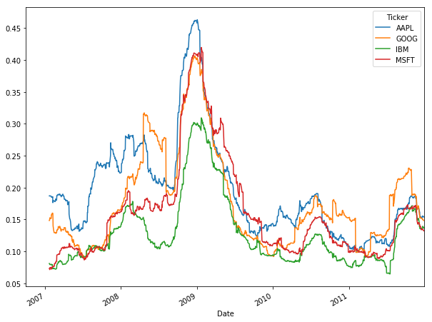
The volatility is calculated by taking a rolling window standard deviation on the percentage change in a stock. You can clearly see this in the code because you pass daily_pct_change and the min_periods to rolling_std().
Note that the size of the window can and will change the overall result: if you take the window wider and make min_periods larger, your result will become less representative. If you make it smaller and make the window more narrow, the result will come closer to the standard deviation.
Considering all of this, you see that it's definitely a skill to get the right window size based upon the data sampling frequency.
Ordinary Least-Squares Regression (OLS)
After all of the calculations, you might also perform a maybe more statistical analysis of your financial data, with a more traditional regression analysis, such as the Ordinary Least-Squares Regression (OLS).
To do this, you have to make use of the statsmodels library, which not only provides you with the classes and functions to estimate many different statistical models but also allows you to conduct statistical tests and perform statistical data exploration.
Note that you could indeed to the OLS regression with Pandas, but that the ols module is now deprecated and will be removed in future versions. It is therefore wise to use the statsmodels package.
Note that you add [1:] to the concatenation of the AAPL and MSFT return data so that you don't have any NaN values that can interfere with your model.
Things to look out for when you're studying the result of the model summary are the following:
- The
Dep. Variable, which indicates which variable is the response in the model - The
Model, in this case, isOLS. It's the model you're using in the fit - Additionally, you also have the
Methodto indicate how the parameters of the model were calculated. In this case, you see that this is set atLeast Squares.
Up until now, you haven't seen much new information. You have basically set all of these in the code that you ran in the DataCamp Light chunk. However, there are also other things that you could find interesting, such as:
- The number of observations (
No. Observations). Note that you could also derive this with the Pandas package by using theinfo()function. Runreturn_data.info()in the IPython console of the DataCamp Light chunk above to confirm this. - The degree of freedom of the residuals (
DF Residuals) - The number of parameters in the model, indicated by
DF Model; Note that the number doesn't include the constant termXwhich was defined in the code above.
This was basically the whole left column that you went over. The right column gives you some more insight into the goodness of the fit. You see, for example:
R-squared, which is the coefficient of determination. This score indicates how well the regression line approximates the real data points. In this case, the result is0.280. In percentages, this means that the score is at 28%. When the score is 0%, it indicates that the model explains none of the variability of the response data around its mean. Of course, a score of 100% indicates the opposite.- You also see the
Adj. R-squaredscore, which at first sight gives the same number. However, the calculation behind this metric adjusts the R-Squared value based on the number of observations and the degrees-of-freedom of the residuals (registered inDF Residuals). The adjustment in this case hasn't had much effect, as the result of the adjusted score is still the same as the regular R-squared score. - The
F-statisticmeasures how significant the fit is. It is calculated by dividing the mean squared error of the model by the mean squared error of the residuals. The F-statistic for this model is514.2. - Next, there's also the
Prob (F-statistic), which indicates the probability that you would get the result of theF-statistic, given the null hypothesis that they are unrelated. - The
Log-likelihoodindicates the log of the likelihood function, which is, in this case3513.2. - The
AICis the Akaike Information Criterion: this metric adjusts the log-likelihood based on the number of observations and the complexity of the model. The AIC of this model is-7022. - Lastly, the
BICor the Bayesian Information Criterion, is similar to the AIC that you just have seen, but it penalizes models with more parameters more severely. Given the fact that this model only has one parameter (checkDF Model), the BIC score will be the same as the AIC score.
Below the first part of the model summary, you see reports for each of the model's coefficients:
- The estimated value of the coefficient is registered at
coef. std erris the standard error of the estimate of the coefficient.- There's also the t-statistic value, which you'll find under
t. This metric is used to measure how statistically significant a coefficient is. P > |t|indicates the null-hypothesis that the coefficient = 0 is true. If it is less than the confidence level, often 0.05, it indicates that there is a statistically significant relationship between the term and the response. In this case, you see that the constant has a value of0.198, whileAAPLis set at0.000.
Lastly, there is a final part of the model summary in which you'll see other statistical tests to assess the distribution of the residuals:
Omnibus, which is the Omnibus D'Angostino's test: it provides a combined statistical test for the presence of skewness and kurtosis.- The
Prob(Omnibus)is theOmnibusmetric turned into a probability. - Next, the
Skewor Skewness measures the symmetry of the data about the mean. - The
Kurtosisgives an indication of the shape of the distribution, as it compares the amount of data close to the mean with those far away from the mean (in the tails). Durbin-Watsonis a test for the presence of autocorrelation, and theJarque-Berais another test of the skewness and kurtosis. You can also turn the result of this test into a probability, as you can see inProb (JB).- Lastly, you have the
Cond. No, which tests the multicollinearity.
You can plot the Ordinary Least-Squares Regression with the help of Matplotlib:

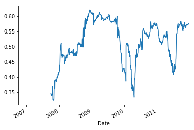
Note that you can also use the rolling correlation of returns as a way to crosscheck your results. You can handily make use of the Matplotlib integration with Pandas to call the plot() function on the results of the rolling correlation:
Building a Trading Strategy with Python
Now that you have done some primary analyses to your data, it's time to formulate your first trading strategy; But before you go into all of this, why not first get to know some of the most common trading strategies? After a short introduction, you'll undoubtedly move on more easily your trading strategy.
Common Trading Strategies
From the introduction, you'll still remember that a trading strategy is a fixed plan to go long or short in markets, but much more information you didn't really get yet; In general, there are two common trading strategies: the momentum strategy and the reversion strategy.
Firstly, the momentum strategy is also called divergence or trend trading. When you follow this strategy, you do so because you believe the movement of a quantity will continue in its current direction. Stated differently, you believe that stocks have momentum or upward or downward trends, that you can detect and exploit.
Some examples of this strategy are the moving average crossover, the dual moving average crossover, and turtle trading:
- The moving average crossover is when the price of an asset moves from one side of a moving average to the other. This crossover represents a change in momentum and can be used as a point of making the decision to enter or exit the market. You'll see an example of this strategy, which is the “hello world” of quantitative trading later on in this tutorial.
- The dual moving average crossover occurs when a short-term average crosses a long-term average. This signal is used to identify that momentum is shifting in the direction of the short-term average. A buy signal is generated when the short-term average crosses the long-term average and rises above it, while a sell signal is triggered by a short-term average crossing long-term average and falling below it.
- Turtle trading is a popular trend following strategy that was initially taught by Richard Dennis. The basic strategy is to buy futures on a 20-day high and sell on a 20-day low.
Secondly, the reversion strategy, which is also known as convergence or cycle trading. This strategy departs from the belief that the movement of a quantity will eventually reverse. This might seem a little bit abstract, but will not be so anymore when you take the example. Take a look at the mean reversion strategy, where you actually believe that stocks return to their mean and that you can exploit when it deviates from that mean.
That already sounds a whole lot more practical, right?
Another example of this strategy, besides the mean reversion strategy, is the pairs trading mean-reversion, which is similar to the mean reversion strategy. Whereas the mean reversion strategy basically stated that stocks return to their mean, the pairs trading strategy extends this and states that if two stocks can be identified that have a relatively high correlation, the change in the difference in price between the two stocks can be used to signal trading events if one of the two moves out of correlation with the other. That means that if the correlation between two stocks has decreased, the stock with the higher price can be considered to be in a short position. It should be sold because the higher-priced stock will return to the mean. The lower-priced stock, on the other hand, will be in a long position because the price will rise as the correlation will return to normal.
Besides these two most frequent strategies, there are also other ones that you might come across once in a while, such as the forecasting strategy, which attempts to predict the direction or value of a stock, in this case, in subsequent future time periods based on certain historical factors. There's also the High-Frequency Trading (HFT) strategy, which exploits the sub-millisecond market microstructure.
That's all music for the future for now; Let's focus on developing your first trading strategy for now!
A Simple Trading Strategy
As you read above, you'll start with the “hello world” of quantitative trading: the moving average crossover. The strategy that you'll be developing is simple: you create two separate Simple Moving Averages (SMA) of a time series with differing lookback periods, let's say, 40 days and 100 days. If the short moving average exceeds the long moving average then you go long, if the long moving average exceeds the short moving average then you exit.
Remember that when you go long, you think that the stock price will go up and will sell at a higher price in the future (= buy signal); When you go short, you sell your stock, expecting that you can buy it back at a lower price and realize a profit (= sell signal).
This simple strategy might seem quite complex when you're just starting out, but let's take this step by step:
- First define your two different lookback periods: a short window and a long window. You set up two variables and assign one integer per variable. Make sure that the integer that you assign to the short window is shorter than the integer that you assign to the long window variable!
- Next, make an empty
signalsDataFrame, but do make sure to copy the index of youraapldata so that you can start calculating the daily buy or sell signal for youraapldata. - Create a column in your empty
signalsDataFrame that is namedsignaland initialize it by setting the value for all rows in this column to0.0. - After the preparatory work, it's time to create the set of short and long simple moving averages over the respective long and short time windows. Make use of the
rolling()function to start your rolling window calculations: within the function, specify thewindowand themin_period, and set thecenterargument. In practice, this will result in arolling()function to which you have passed eithershort_windoworlong_window,1as the minimum number of observations in the window that are required to have a value, andFalse, so that the labels are not set at the center of the window. Next, don't forget to also chain themean()function so that you calculate the rolling mean. - After you have calculated the mean average of the short and long windows, you should create a signal when the short moving average crosses the long moving average, but only for the period greater than the shortest moving average window. In Python, this will result in a condition:
signals['short_mavg'][short_window:] > signals['long_mavg'][short_window:]. Note that you add the[short_window:]to comply with the condition “only for the period greater than the shortest moving average window”. When the condition is true, the initialized value0.0in thesignalcolumn will be overwritten with1.0. A “signal” is created! If the condition is false, the original value of0.0will be kept and no signal is generated. You use the NumPywhere()function to set up this condition. Much the same like you read just now, the variable to which you assign this result issignals['signal'][short_window], because you only want to create signals for the period greater than the shortest moving average window! - Lastly, you take the difference of the signals in order to generate actual trading orders. In other words, in this column of your
signalsDataFrame, you'll be able to distinguish between long and short positions, whether you're buying or selling stock.
Try all of this out in the DataCamp Light chunk below:
This wasn't too hard, was it? Print out the signals DataFrame and inspect the results. Important to grasp here is what the positions and the signal columns mean in this DataFrame. You'll see that it will become very important when you move on!
When you have taken the time to understand the results of your trading strategy, quickly plot all of this (the short and long moving averages, together with the buy and sell signals) with Matplotlib:
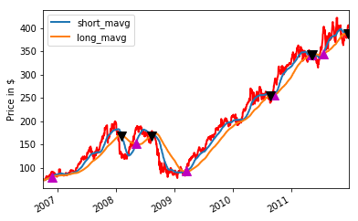
The result is pretty cool, isn't it?
Backtesting the Trading Strategy
Now that you've got your trading strategy at hand, it's a good idea to also backtest it and calculate its performance. But right before you go deeper into this, you might want to know just a little bit more about the pitfalls of backtesting, what components are needed in a backtester and what Python tools you can use to backtest your simple algorithm.
If, however, you're already well up to date, you can simply move on to the implementation of your backtester!
Backtesting Pitfalls
Backtesting is, besides just “testing a trading strategy”, testing the strategy on relevant historical data to make sure that it's an actual viable strategy before you start making moves. With backtesting, a trader can simulate and analyze the risk and profitability of trading with a specific strategy over a period of time. However, when you're backtesting, it's a good idea to keep in mind that there are some pitfalls, which might not be obvious to you when you're just starting out.
For example, there are external events, such as market regime shifts, which are regulatory changes or macroeconomic events, which definitely influence your backtesting. Also, liquidity constraints, such as the ban of short sales, could affect your backtesting heavily.
Next, there are pitfalls which you might introduce yourself when you, for example, overfit a model (optimization bias), when you ignore strategy rules because you think it's better like that (interference), or when you accidentally introduce information into past data (lookahead bias).
These are just a few pitfalls that you need to take into account mainly after this tutorial, when you go and make your own strategies and backtest them.
Backtesting Components
Besides the pitfalls, it's good to know that your backtester usually consists of some four essential components, which should usually present in every backtester:
- A data handler, which is an interface to a set of data,
- A strategy, which generates a signal to go long or go short based on the data,
- A portfolio, which generates orders and manages Profit & Loss (also known as “PnL”), and
- An execution handler, which sends the order to the broker and receives the “fills” or signals that the stock has been bought or sold.
Besides these four components, there are many more that you can add to your backtester, depending on the complexity. You can definitely go a lot further than just these four components. However, for this beginner tutorial, you'll just focus on getting these basic components to work in your code.
Python Tools
To implement the backtesting, you can make use of some other tools besides Pandas, which you have already used extensively in the first part of this tutorial to perform some financial analyses on your data. Apart from Pandas, there is, for example, also NumPy and SciPy, which provide, vectorization, optimization and linear algebra routines which you can use when you're developing trading strategies.
Also Scikit-Learn, the Python Machine Learning library, can come in handy when you're working with forecasting strategies, as they offer everything you need to create regression and classification models. For an introduction to this library, consider DataCamp's Supervised Learning With Scikit-Learn course. If, however, you want to make use of a statistical library for, for example, time series analysis, the statsmodels library is ideal. You briefly used this library already in this tutorial when you were performing the Ordinary Least-Squares Regression (OLS).
Lastly, there's also the IbPy and ZipLine libraries. The former offers you a Python API for the Interactive Brokers online trading system: you'll get all the functionality to connect to Interactive Brokers, request stock ticker data, submit orders for stocks,… The latter is an all-in-one Python backtesting framework that powers Quantopian, which you'll use in this tutorial.
Implementation of a Simple Backtester
As you read above, a simple backtester consists of a strategy, a data handler, a portfolio and an execution handler. You have already implemented a strategy above, and you also have access to a data handler, which is the pandas-datareader or the Pandas library that you use to get your saved data from Excel into Python. The components that are still left to implement are the execution handler and the portfolio.
However, since you're just starting out, you'll not focus on implementing an execution handler just yet. Instead, you'll see below how you can get started on creating a portfolio which can generate orders and manages the profit and loss:
- First off, you'll create set a variable
initial_capitalto set your initial capital and a new DataFramepositions. Once again, you copy the index from another DataFrame; In this case, this is thesignalsDataFrame because you want to consider the time frame for which you have generated the signals. - Next, you create a new column
AAPLin the DataFrame. On the days that the signal is 1 and the short moving average crosses the long moving average (for the period greater than the shortest moving average window), you'll buy a 100 shares. The days on which the signal is 0, the final result will be 0 as a result of the operation100*signals['signal']. - A new DataFrame
portfoliois created to store the market value of an open position. - Next, you create a DataFrame that stores the differences in positions (or number of stock)
- Then the real backtesting begins: you create a new column to the
portfolioDataFrame with nameholdings, which stores the value of the positions or shares you have bought, multiplied by the ‘Adj Close' price. - Your
portfolioalso contains acashcolumn, which is the capital that you still have left to spend: it is calculated by taking yourinitial_capitaland subtracting your holdings (the price that you paid for buying stock). - You'll also add a
totalcolumn to yourportfolioDataFrame, which contains the sum of your cash and the holdings that you own, and - Lastly, you also add a
returnscolumn to your portfolio, in which you'll store the returns
As a last exercise for your backtest, visualize the portfolio value or portfolio['total'] over the years with the help of Matplotlib and the results of your backtest:
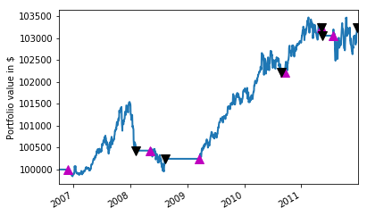
Note that, for this tutorial, the Pandas code for the backtester as well as the trading strategy has been composed in such a way that you can easily walk through it in an interactive way. In a real-life application, you might opt for a more object-oriented design with classes, which contain all the logic. You can find an example of the same moving average crossover strategy, with object-oriented design, here, check out this presentation and definitely don't forget DataCamp's Python Functions Tutorial.
Backtesting with Zipline & Quantopian
You have seen now how you can implement a backtester with the Python's popular data manipulation package Pandas. However, you can also see that it's easy to make mistakes and that this might not be the most fail-safe option to use every time: you need to build most of the components from scratch, even though you already leverage Pandas to get your results.
That's why it's common to use a backtesting platform, such as Quantopian, for your backtesters. Quantopian is a free, community-centered, hosted platform for building and executing trading strategies. It's powered by zipline, a Python library for algorithmic trading. You can use the library locally, but for the purpose of this beginner tutorial, you'll use Quantopian to write and backtest your algorithm. Before you can do this, though, make sure that you first sign up and log in.
Next, you can get started pretty easily. Click “New Algorithm” to start writing up your trading algorithm or select one of the examples that has already been coded up for you to get a better feeling of what you're exactly dealing with :)
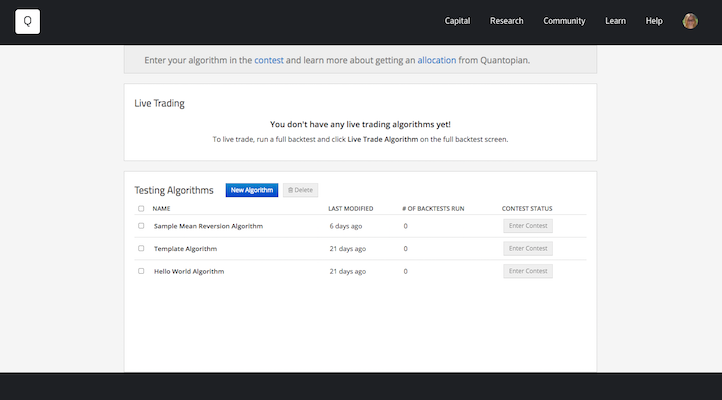
Let's start simple and make a new algorithm, but still following our simple example of the moving average crossover, which is the standard example that you find in the zipline Quickstart guide.
It so happens that this example is very similar to the simple trading strategy that you implemented in the previous section. You see, though, that the structure in the code chunk below and in the screenshot above is somewhat different than what you have seen up until now in this tutorial, namely, you have two definitions that you start working from, namely initialize() and handle_data():
def initialize(context):
    context.sym = symbol('AAPL')
    context.i = 0


def handle_data(context, data):
    # Skip first 300 days to get full windows
    context.i += 1
    if context.i < 300:
        return

    # Compute averages
    # history() has to be called with the same params
    # from above and returns a pandas dataframe.
    short_mavg = data.history(context.sym, 'price', 100, '1d').mean()
    long_mavg = data.history(context.sym, 'price', 300, '1d').mean()

    # Trading logic
    if short_mavg > long_mavg:
        # order_target orders as many shares as needed to
        # achieve the desired number of shares.
        order_target(context.sym, 100)
    elif short_mavg < long_mavg:
        order_target(context.sym, 0)

    # Save values for later inspection
    record(AAPL=data.current(context.sym, "price"),
           short_mavg=short_mavg,
           long_mavg=long_mavg)
The first function is called when the program is started and performs one-time startup logic. As an argument, the initialize() function takes a context, which is used to store the state during a backtest or live trading and can be referenced in different parts of the algorithm, as you can see in the code below; You see that context comes back, among others, in the definition of the first moving average window. You see that you assign the result of the lookup of a security (stock in this case) by its symbol, (AAPL in this case) to context.security.
The handle_data() function is called once per minute during simulation or live-trading to decide what orders, if any, should be placed each minute. The function requires context and data as input: the context is the same as the one that you read about just now, while the data is an object that stores several API functions, such as current() to retrieve the most recent value of a given field(s) for a given asset(s) or history() to get trailing windows of historical pricing or volume data. These API functions don't come back in the code below and are not in the scope of this tutorial.
Note That the code that you type into the Quantopian console will only work on the platform itself and not in your local Jupyter Notebook, for example!
You'll see that the data object allows you to retrieve the price, which is the forward-filled, returning last known price, if there is one. If there is none, an NaN value will be returned.
Another object that you see in the code chunk above is the portfolio, which stores important information about…. Your portfolio. As you can see in the piece of code context.portfolio.positions, this object is stored in the context and is then also accessible in the core functions that context has to offer to you as a user. Note that the positions that you just read about, store Position objects and include information such as the number of shares and price paid as values. Additionally, you also see that the portfolio also has a cash property to retrieve the current amount of cash in your portfolio and that the positions object also has an amount property to explore the whole number of shares in a certain position.
The order_target() places an order to adjust a position to a target number of shares. If there is no existing position in the asset, an order is placed for the full target number. If there is a position in the asset, an order is placed for the difference between the target number of shares or contracts and the number currently held. Placing a negative target order will result in a short position equal to the negative number specified.
Tip: if you have any more questions about the functions or objects, make sure to check the Quantopian Help page, which contains more information about all (and much more) that you have briefly seen in this tutorial.
When you have created your strategy with the initialize() and handle_data() functions (or copy-pasted the above code) into the console on the left-hand side of your interface, just press the “Build Algorithm” button to build the code and run a backtest. If you press the “Run Full Backtest” button, a full backtest is run, which is basically the same as the one that you run when you build the algorithm, but you'll be able to see a lot more in detail. The backtesting, whether ‘simple' or full, can take a while; Make sure to keep an eye out on the progress bar on top of the page!
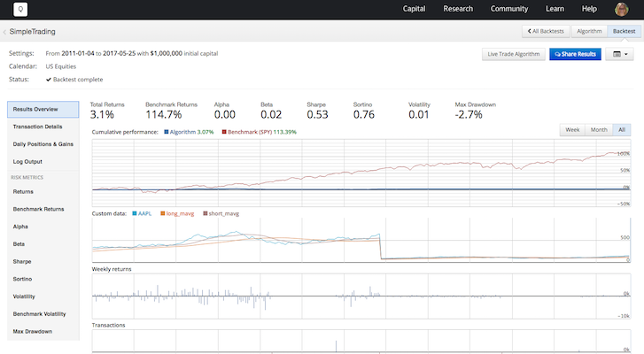
You can find more information on how to get started with Quantopian here.
Note that Quantopian is an easy way to get started with zipline, but that you can always move on to using the library locally in, for example, your Jupyter notebook.
Improving the Trading Strategy
You have successfully made a simple trading algorithm and performed backtests via Pandas, Zipline and Quantopian. It's fair to say that you've been introduced to trading with Python. However, when you have coded up the trading strategy and backtested it, your work doesn't stop yet; You might want to improve your strategy. There are one or more algorithms may be used to improve the model on a continuous basis, such as KMeans, k-Nearest Neighbors (KNN), Classification or Regression Trees and the Genetic Algorithm. This will be the topic of a future DataCamp tutorial.
Apart from the other algorithms you can use, you saw that you can improve your strategy by working with multi-symbol portfolios. Just incorporating one company or symbol into your strategy often doesn't really say much. You'll also see this coming back in the evaluation of your moving average crossover strategy. Other things that you can add or do differently is using a risk management framework or use event-driven backtesting to help mitigate the lookahead bias that you read about earlier. There are still many other ways in which you could improve your strategy, but for now, this is a good basis to start from!
Evaluating Moving Average Crossover Strategy
Improving your strategy doesn't mean that you're finished just yet! You can easily use Pandas to calculate some metrics to further judge your simple trading strategy. First, you can use the Sharpe ratio to get to know whether your portfolio's returns are the result of the fact that you decided to make smart investments or to take a lot of risks.
The ideal situation is, of course, that the returns are considerable but that the additional risk of investing is as small as possible. That's why, the greater the portfolio's Sharpe ratio, the better: the ratio between the returns and the additional risk that is incurred is quite OK. Usually, a ratio greater than 1 is acceptable by investors, 2 is very good and 3 is excellent.
Let's see how your algorithm does!
Note that the risk free rate that is excluded in the definition of the Sharpe ratio for this tutorial and that the Sharpe ratio is usually not considered as a standalone: it's usually compared to other stocks. The best way to approach this issue is thus by extending your original trading strategy with more data (from other companies)!
Next, you can also calculate a Maximum Drawdown, which is used to measure the largest single drop from peak to bottom in the value of a portfolio, so before a new peak is achieved. In other words, the score indicates the risk of a portfolio chosen based on a certain strategy.
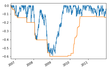
Note that you set min_periods to 1 because you want to let the first 252 days data have an expanding window.
Next up is the Compound Annual Growth Rate (CAGR), which provides you with a constant rate of return over the time period. In other words, the rate tells you what you really have at the end of your investment period. You can calculate this rate by first dividing the investments ending value (EV) by the investment's beginning value (BV). You raise the result to the power of 1/n, where n is the number of periods. You subtract 1 from the consequent result and there's your CAGR!
Maybe a formula is more clear: \[(EV/BV)^{1/n} - 1\]
Note that, in the code chunk below, you'll see that you consider days, so your 1 is adjusted to 365 days (which is equal to 1 year).
Besides these two metrics, there are also many others that you could consider, such as the distribution of returns, trade-level metrics, …
What Now?
Well done, you've made it through this Python Finance introduction tutorial! You've covered a lot of ground, but there's still so much more for you to discover! Start by taking DataCamp's Intro to Python for Finance course to learn more of the basics.
You should also check out Yves Hilpisch's Python For Finance book, which is a great book for those who already have gathered some background into Finance, but not so much in Python. “Mastering Pandas for Data Science” by Michael Heydt is also recommended for those who want to get started with Finance in Python! Also make sure to check out Quantstart's articles for guided tutorials on algorithmic trading and this complete series on Python programming for finance.
If you're more interested in continuing your journey into finance with R, consider taking Datacamp's Quantitative Analyst with R track. And in the meantime, keep posted for our second post on starting finance with Python and check out the Jupyter notebook of this tutorial.
The information provided on this site is not financial advice and none of the authors are financial professionals. The material provided on this Website should be used for informational purposes only and in no way should be relied upon for financial advice. We make no representations as to accuracy, completeness, suitability, or validity, of any information. We will not be liable for any errors, omissions, or any losses, injuries, or damages arising from its display or use. All information is provided AS IS with no warranties, and confers no rights. Also, note that such material is not updated regularly and some of the information may not, therefore, be current. Please be sure to consult your own financial advisor when making decisions regarding your financial management. The ideas and strategies mentioned in this blog should never be used without first assessing your own personal and financial situation, or without consulting a financial professional.
