Course
Cluster Analysis in R
4 hr
44.1K
Imagine that you are a Data Scientist working for a retail company. Your boss requests that you segment customers into the following groups: low, average, medium, or platinum customers based on spending behavior for targeted marketing purposes and product recommendations.
Knowing that there is no such historical label associated with those customers, how is it possible to categorize them?
This is where clustering can help. It is an unsupervised machine learning technique used to group unlabeled data into similar categories.
This tutorial will focus more on the hierarchical clustering approach, one of the many techniques in unsupervised machine learning. It will start by providing an overview of what hierarchical clustering is, before comparing it to some existing techniques.
Then, it will walk you through a step-by-step implementation in Python using the popular Scipy library.
A hierarchical clustering approach is based on the determination of successive clusters based on previously defined clusters. It's a technique aimed more toward grouping data into a tree of clusters called dendrograms, which graphically represents the hierarchical relationship between the underlying clusters.
Hierarchical clustering is a powerful algorithm, but it is not the only one out there, and each type of clustering comes with its set of advantages and drawbacks.
Let’s understand how it compares to other types of clustering, such as K-means and model-based clustering. Many more techniques exist, but these two, in addition to hierarchical clustering, are widely used and provide a framework to help better understand the others.
You can learn more about clustering in machine learning in our separate article, covering five essential clustering algorithms.
Unlike Hierarchical clustering, K-means clustering seeks to partition the original data points into “K” groups or clusters where the user specifies “K” in advance.
The general idea is to look for clusters that minimize the squared Euclidean distance of all the points from the centers over all attributes (variables or features) and merge those individuals in an iterative manner.
Our K-means Clustering in Python with Scikit-learn tutorial will help you understand the inner workings of K-means clustering with an interesting case study.
Despite its limitations, k-means clustering is still a popular method due to its ease of use and computational efficiency. It is frequently used as a reference point for comparing the performance of other clustering techniques.
Both K-means and hierarchical clustering techniques use a distance matrix to represent the distances between all the points in the dataset. Model-based clustering, on the other hand, applies statistical techniques to identify clusters in the data. Below is the general process:
Hierarchical clustering has a variety of applications in our day-to-day life, including (but by no means limited to) biology, image processing, marketing, economics, and social network analysis.
The clustering of DNA sequences is one of the biggest challenges in bioinformatics.
Biologists can leverage hierarchical clustering to study genetic relationships between organisms to classify those organisms into taxonomic groups. This is beneficial for quick analysis and visualization of the underlying relationships.
Hierarchical clustering can be performed in image processing to group similar regions or pixels of an image in terms of color, intensity, or other features. This can be useful for further tasks such as image segmentation, image classification, and object recognition.
Marketing specialists can use hierarchical clustering to draw a hierarchy between different types of customers based on their purchasing habits for better marketing strategies and product recommendations. For instance, different products in retails can be recommended to customers whether they are low, medium, or high spenders.
Social networks are a great source of valuable information when exploited efficiently. Hierarchical clustering can be used to identify groups or communities and to understand their relationships to each other and the structure of the network as a whole.
In this section, we will look at three main concepts. The steps of the hierarchical algorithm, a highlight of the two types of hierarchical clustering (agglomerative and divisive), and finally, some techniques to choose the right distance measure.
The hierarchical clustering algorithm employs the use of distance measures to generate clusters. This generation process involves the following main steps:
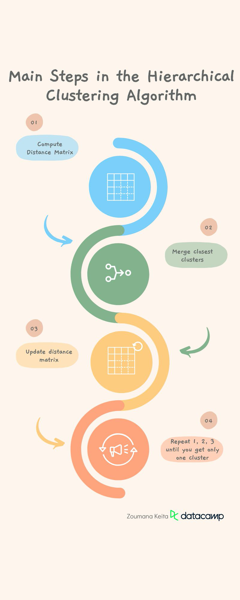
Preprocess the data by removing missing data and applying any additional tasks that make the data as clean as possible. This step is a more general one for most of the machine learning tasks.
1. Compute the distance matrix containing the distance between each pair of data points using a particular distance metric such as Euclidean distance, Manhattan distance, or cosine similarity. But the default distance metric is the Euclidean one.
2.Merge the two clusters that are the closest in distance.
3. Update the distance matrix with regard to the new clusters.
4. Repeat steps 1, 2, and 3 until all the clusters are merged together to create a single cluster.
We can consider agglomerative and divisive clustering as mirrors of each other. Let’s have a better look at how each one operates, along with a hierarchical clustering example and graphical visualization.
This first scenario corresponds to the approach explained above. It starts by considering each observation as a singleton cluster (cluster with only one data point). Then iteratively merges clusters until only one cluster is obtained. This process is also known as the bottom-up approach.
As showing in the illustration below:
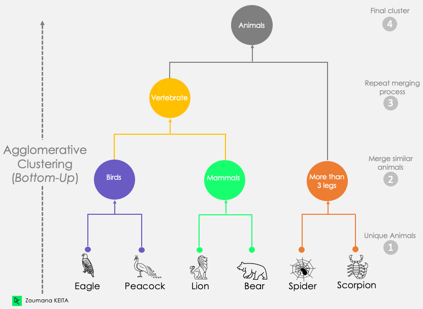
Dendrogram of Agglomerative Clustering Approach
On the other hand, divisive clustering is top-down because it starts by considering all the data points as a unique cluster. Then it separates them until all the data points are unique.
From this divisive approach graphic:
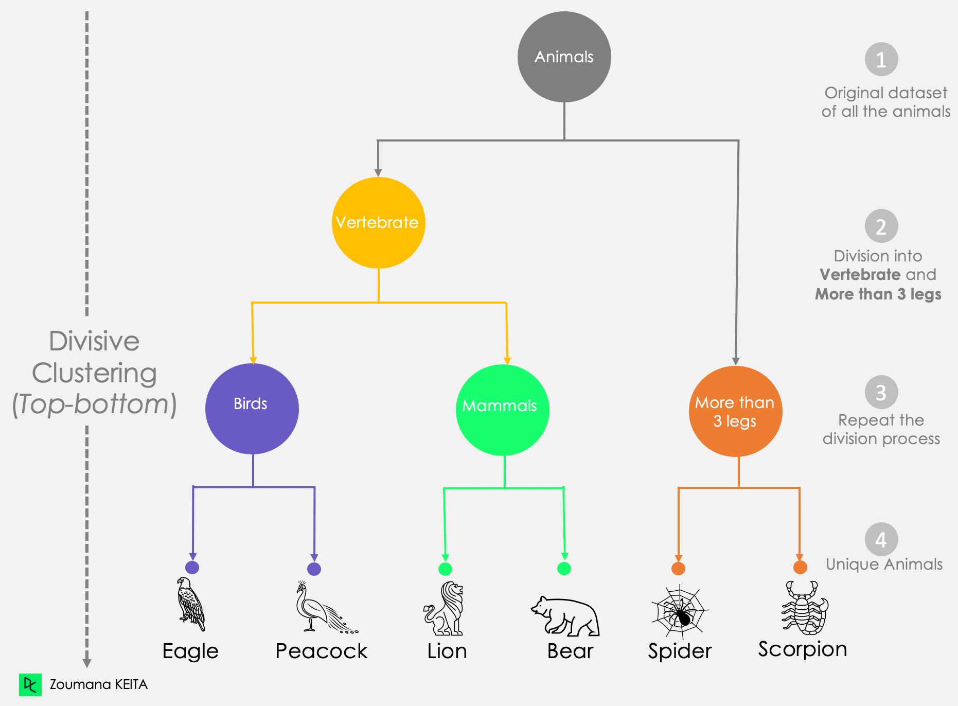
Dendrogram of Divisive Clustering Approach
Your choice of distance measure is a critical step in clustering, and it depends on the problem you’re trying to solve. Considering the following scenario, we could cluster students based on any number of approaches such as their:
These are all valid clusters but differ in meaning.
Even though Euclidean distance is the most common distance used in most clustering software, other distance measures such as Manhattan distance, Canberra distance, Pearson or Spearman correlation, and Minkowski distance exist.
The previously mentioned distances are related to items. In this section, we will cover three standard ways (not exhaustive) to measure the nearest pair of clusters before merging them: (1) Single linkage, (2) Complete linkage, and (3) Average linkage.
From all the pairwise distances between the items in the two clusters C1 and C2, the single linkage takes the distance between the clusters as the minimum distance.
Distance (C1, C2) = Min { d(i, j), where item i is within C1, and item j is within C2}
Out of all the pairs of items from the two clusters, the ones highlighted in green have the minimum distance.
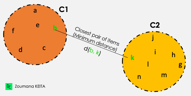
Single linkage illustration
From all the pairwise distances between the items in the two clusters C1 and C2, the single linkage takes the distance between the clusters as the maximum distance.
Distance (C1, C2) = Max { d(i, j), where item i is within C1, and item j is within C2}
Out of all the pairs of items from the two clusters, the ones highlighted in green have the maximum distance.
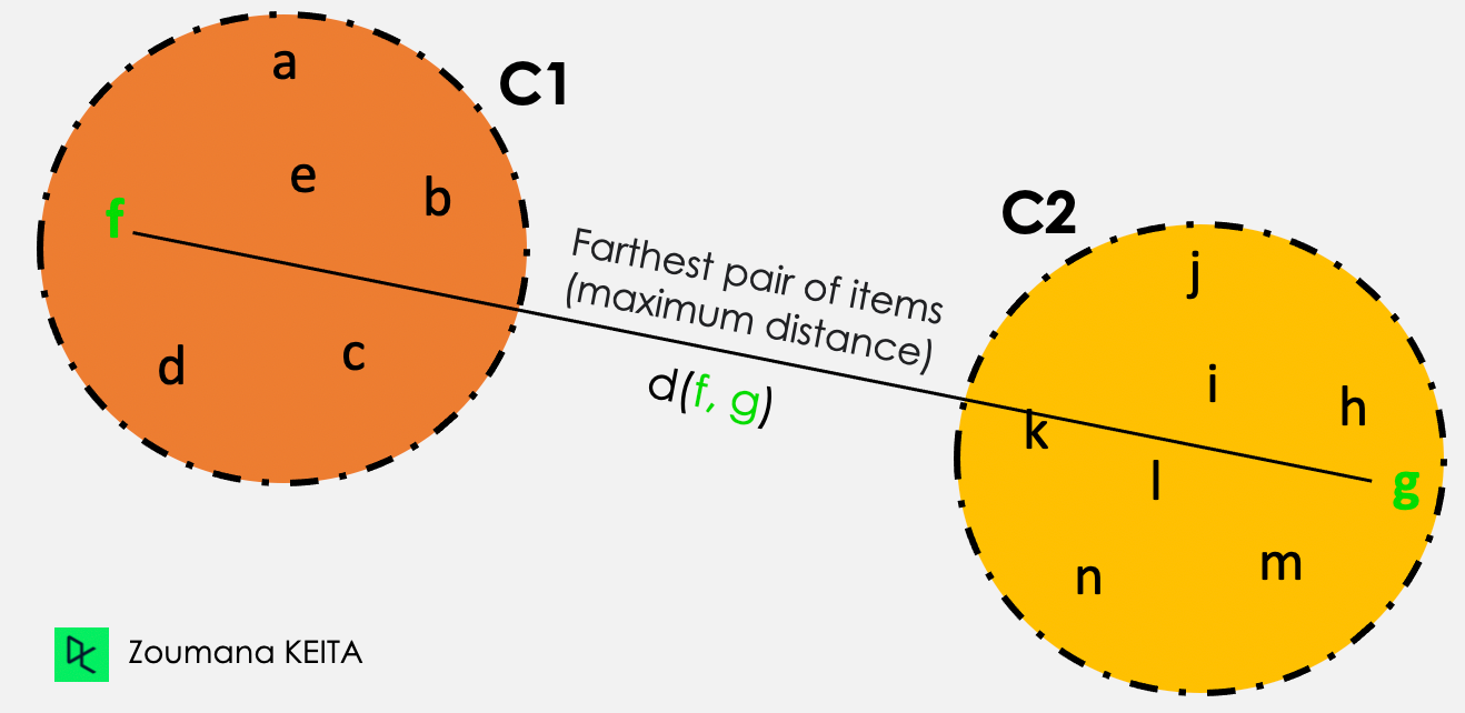
Complete linkage illustration
In the average linkage clustering, the distance between two given clusters C1 and C2 corresponds to the average distances between all pairs of items in the two clusters.
Distance (C1, C2) = Sum{ d(i, j) } / Total Number of distances
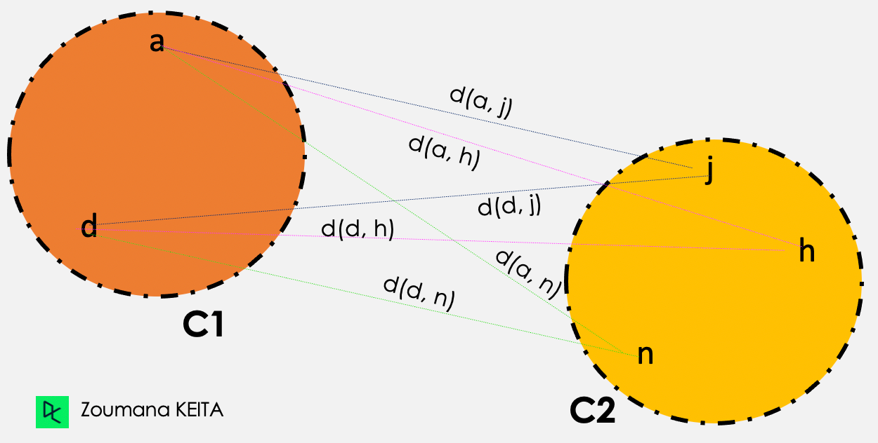
Average linkage illustration
Then the average linkage clustering is performed as follows
d(a,j) + d(a,h) + d(a,n) + d(d,j) + d(d,h) + d(d,n)
—-----------------------------------------------------------, where Total number of distances = 6
Total number of distances
Now you have an understanding of how hierarchical clustering works. In this section, we will focus on the technical implementation using Python.
If you are more interested in performing the implementation with R programming language, our Hierarchical clustering in R tutorial is where to start.
To begin, you will need to have Python installed on your computer, along with the following libraries:
You can install these libraries using pip, the Python package manager as follows:
pip install scikit-learn
pip install pandas

pip install matplotlib seaborn

pip install scipy
Next, let's import the necessary modules and load the dataset. We will use the built-in iris dataset from scikit-learn, which contains information about different types of iris flowers.
To better illustrate the use case, we will be using the Loan Data available on DataLab. All the code in this tutorial is available in this DataLab workbook; you can easily create a copy of your own to run the code in the browser, without having to install any software on your computer.
The data set has 9,500 loans with information on the loan structure, the borrower, and whether the loan was paid back in full. We will get rid of the target column not.fully.paid to meet the unsupervised aspect.
import pandas as pd
loan_data = pd.read_csv("loan_data.csv")
loan_data.head()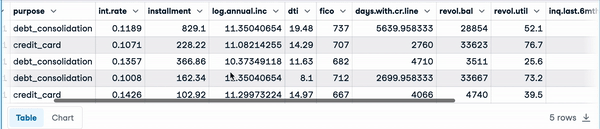 First five rows of the load data
The following instruction shows that the data has 9,578 rows, and 14 columns of numerical types except for purpose, which is object and gives the textual description of the purpose of the load.
loan_data.info() Information about the data
Before the application of the clustering, the data need to be preprocessed to deal with missing information, normalize the column values, and drop irrelevant columns.
From the output below, we notice that there is no missing value in the data.
percent_missing =round(100*(loan_data.isnull().sum())/len(loan_data),2)
percent_missing
Percentage of missing values in the data
We are going to analyze the loan data using all the columns except the following:
The cleaned_data corresponds to the data without the above columns.
cleaned_data = loan_data.drop(['purpose', 'not.fully.paid'], axis=1)
cleaned_data.info()
The image below shows the information of the new data.
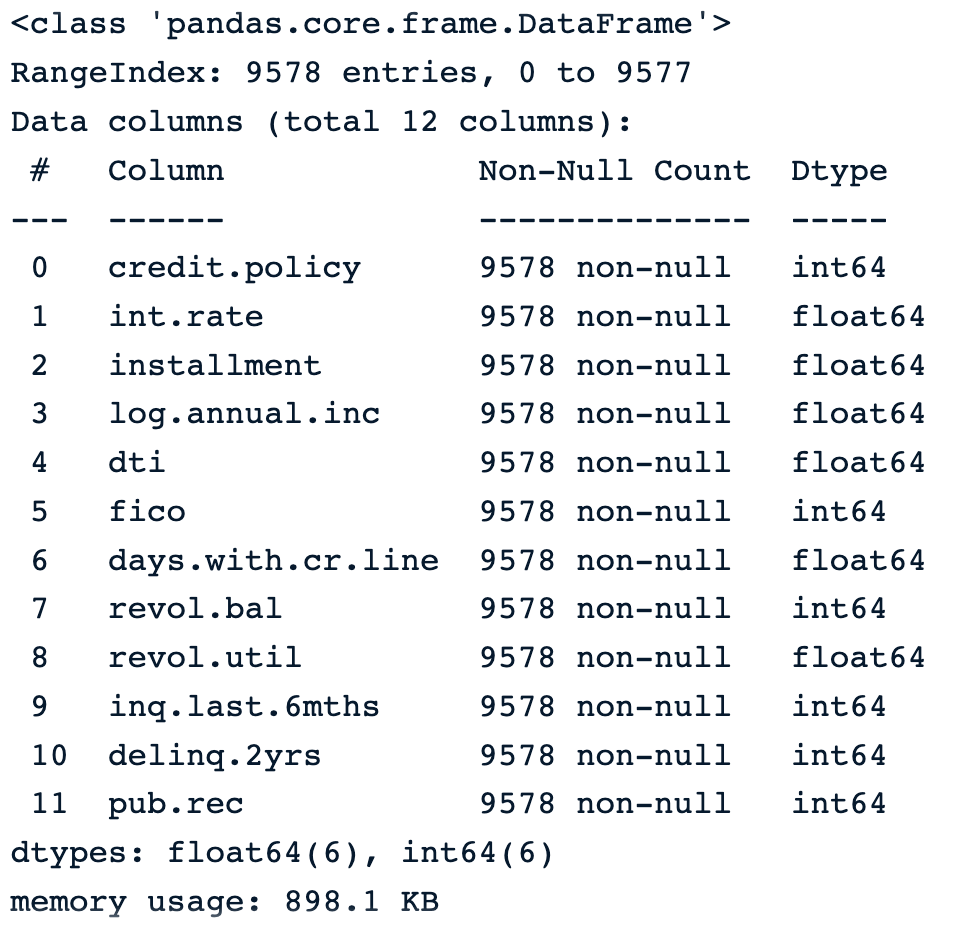
New data without the unwanted columns
One of the weaknesses of hierarchical clustering is that it is sensitive to outliers. The distribution of each variable is given by the boxplot.
def show_boxplot(df):
plt.rcParams['figure.figsize'] = [14,6]
sns.boxplot(data = df, orient="v")
plt.title("Outliers Distribution", fontsize = 16)
plt.ylabel("Range", fontweight = 'bold')
plt.xlabel("Attributes", fontweight = 'bold')

show_boxplot(cleaned_data)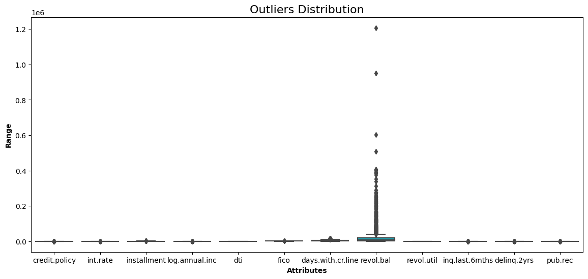
Boxplot of all the variables in the data
The borrower’s revolving balance (revol_bal) is the only attribute with data points far away from the rest.
By using the interquartile range approach, we can remove all such points that lie outside the range defined by the quartiles +/-1.5 * IQR, where IQR is the InterQuartile Range.
This is achieved with the following helper function.
def remove_outliers(data):

df = data.copy()

for col in list(df.columns):

      Q1 = df[str(col)].quantile(0.05)
      Q3 = df[str(col)].quantile(0.95)
      IQR = Q3 - Q1
      lower_bound = Q1 - 1.5*IQR
      upper_bound = Q3 + 1.5*IQR

      df = df[(df[str(col)] >= lower_bound) &

        (df[str(col)] <= upper_bound)]

return df
Then, we can apply the function to the data set.
without_outliers = remove_outliers(cleaned_data)Now we can check the new boxplot and compare it with the one before the removal of the outliers.
show_boxplot(without_outliers)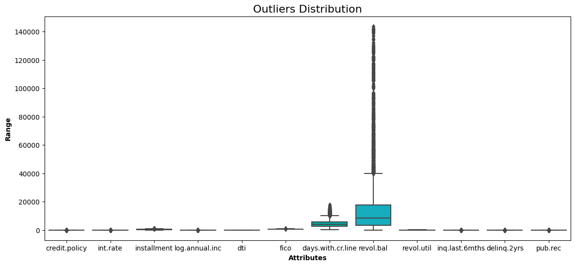
No more data points lie outside the interquartile range.
without_outliers.shapeThe shape of the data is now 9,319 rows and 12 columns. This means that 259 observations were outliers, which have been dropped.
Since hierarchical clustering uses Euclidean distance, which is very sensitive to dealing with variables with different scales, it’s wise to rescale all the variables before computing the distance.
This is done using the StandardScaler class from sklearn.
from sklearn.preprocessing import StandardScaler

data_scaler = StandardScaler()

scaled_data = data_scaler.fit_transform(without_outliers)
scaled_data.shape
The shape of the data remains the same (9,319 rows, 12 columns) because the normalization does not affect the same of the data.
All the requirements are met to dive deep into the implementation of the clustering algorithm.
At this point, we can decide which linkage approach to adopt for the clustering in the method attribute of linkage() method. In this section, we will cover all three linkage techniques using the euclidean distance.
This is achieved with the codes below after importing the relevant libraries.
from scipy.cluster.hierarchy import linkage, dendrogram

complete_clustering = linkage(scaled_data, method="complete", metric="euclidean")
average_clustering = linkage(scaled_data, method="average", metric="euclidean")
single_clustering = linkage(scaled_data, method="single", metric="euclidean")
Once we have computed all the three clusterings, the corresponding dendrograms are shown as follows, starting with the complete clustering
dendrogram(complete_clustering)
plt.show()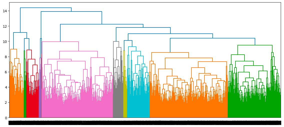
Dendrogram of the complete clustering approach
dendrogram(average_clustering)
plt.show()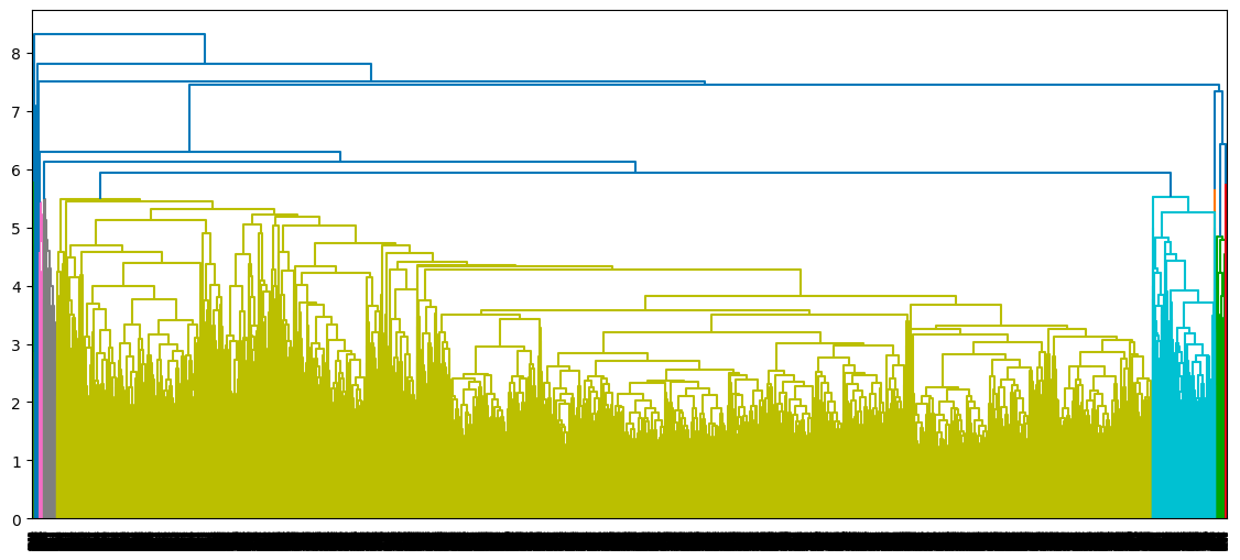
Dendrogram of the average clustering approach
dendrogram(single_clustering)
plt.show()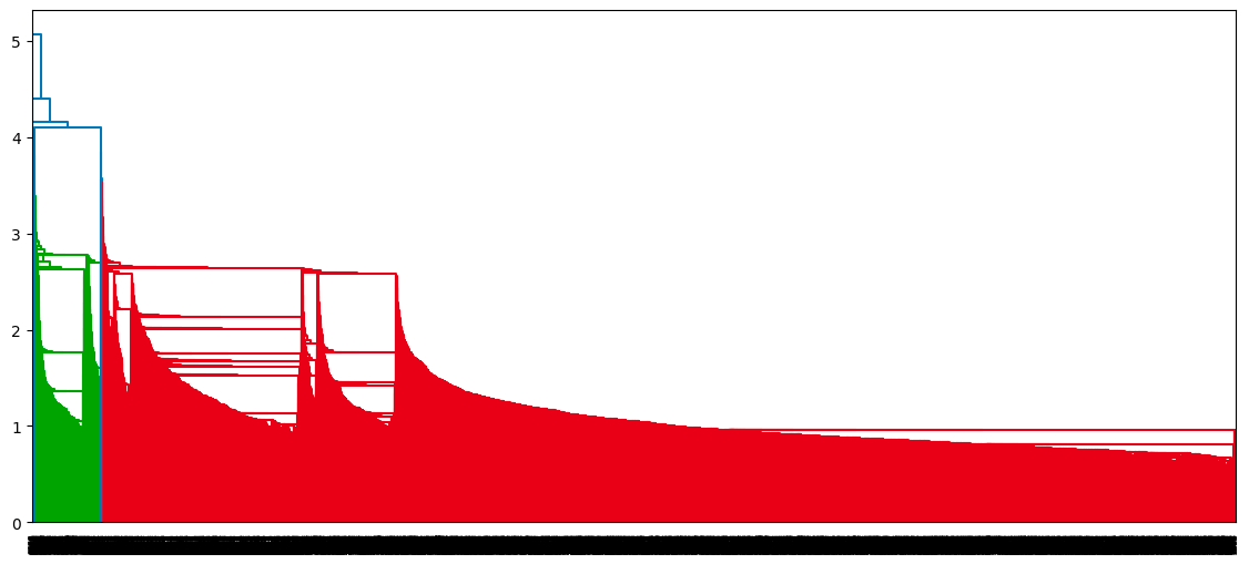
Dendrogram of the single clustering approach
For each linkage approach, how the dendrogram is constructed and every data point ends up into a single cluster.
The optimal number of clusters can be obtained by identifying the highest vertical line that does not intersect with any other clusters (horizontal line). Such a line is found below with a red circle and green check mark.
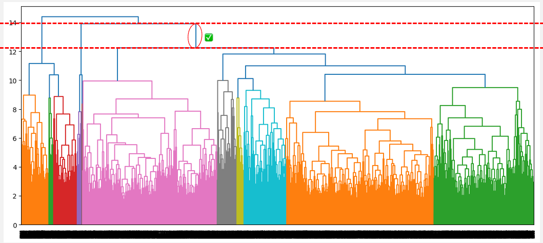
Optimal number of cluster from the highest distance without intersection (complete linkage)
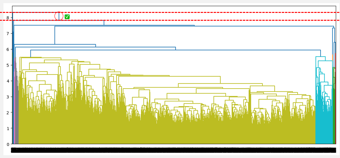
Optimal number of clusters from the highest distance without intersection (average linkage)
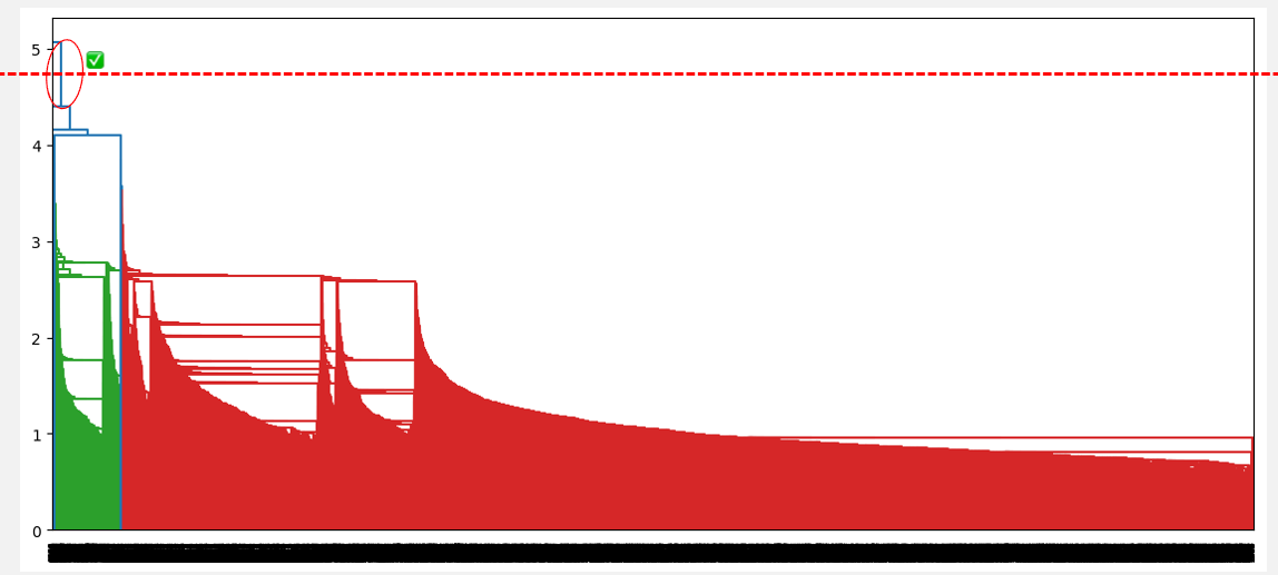
Optimal number of clusters from the highest distance without intersection (single linkage)
From the above observations, the average linkage seems to be the one that provides the best clustering, as opposed to the single and complete linkage, which respectively suggests considering one cluster and three clusters. Also, the optimal cluster number of two corresponds to our prior knowledge about the dataset, which is the two types of borrowers.
Now that we have found the optimal number of clusters let's look at what those clusters mean based on the borrower’s credit score.
cluster_labels = cut_tree(average_clustering, n_clusters=2).reshape(-1, )
without_outliers["Cluster"] = cluster_labels

sns.boxplot(x='Cluster', y='fico', data=without_outliers)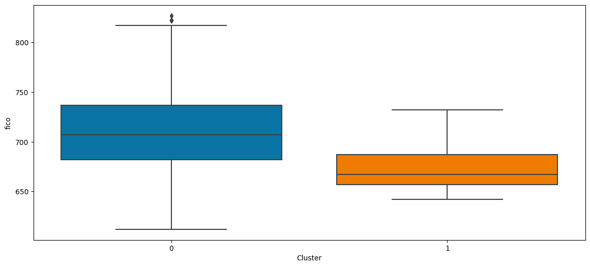
From the above boxplot, we can observe that:
Cluster Analysis in Python can be a good next step to dive deep into K-means and hierarchical clustering using the Scipy library.
This article has covered what hierarchical clustering is, its benefits and weaknesses, and how it compares to k-means and model-based clustering.
We hope the article provides you with the relevant skills to efficiently cluster your unlabeled data for actionable decision-making.
Clustering Courses
Course
Course
blog
Moez Ali
15 min
Tutorial
Kevin Babitz
Tutorial
Kurtis Pykes
Tutorial
Aditya Sharma
Tutorial
DataCamp Team
code-along
George Boorman