Course
In this tutorial, you will learn to perform hierarchical clustering on a dataset in R. If you want to learn about hierarchical clustering in Python, check out our separate article.
Introduction
As the name itself suggests, Clustering algorithms group a set of data points into subsets or clusters. The algorithms' goal is to create clusters that are coherent internally, but clearly different from each other externally. In other words, entities within a cluster should be as similar as possible and entities in one cluster should be as dissimilar as possible from entities in another.
Broadly speaking there are two ways of clustering data points based on the algorithmic structure and operation, namely agglomerative and divisive.
- Agglomerative : An agglomerative approach begins with each observation in a distinct (singleton) cluster, and successively merges clusters together until a stopping criterion is satisfied.
- Divisive : A divisive method begins with all patterns in a single cluster and performs splitting until a stopping criterion is met.
In this tutorial you are going to focus on the agglomerative or bottom-up approach, where you start with each data point as its own cluster and then combine clusters based on some similarity measure. The idea can be easily adapted for divisive methods as well.
The similarity between the clusters is often calculated from the dissimilarity measures like the euclidean distance between two clusters. So the larger the distance between two clusters, the better it is.
There are many distance metrics that you can consider to calculate the dissimilarity measure, and the choice depends on the type of data in the dataset. For example if you have continuous numerical values in your dataset you can use euclidean distance, if the data is binary you may consider the Jaccard distance (helpful when you are dealing with categorical data for clustering after you have applied one-hot encoding). Other distance measures include Manhattan, Minkowski, Canberra etc.
Develop AI Applications
Pre-processing operations for Clustering
There are a couple of things you should take care of before starting.
- Scaling
It is imperative that you normalize your scale of feature values in order to begin with the clustering process. This is because each observations' feature values are represented as coordinates in n-dimensional space (n is the number of features) and then the distances between these coordinates are calculated. If these coordinates are not normalized, then it may lead to false results.
For example, suppose you have data about height and weight of three people: A (6ft, 75kg), B (6ft,77kg), C (8ft,75kg). If you represent these features in a two-dimensional coordinate system, height and weight, and calculate the Euclidean distance between them, the distance between the following pairs would be:
A-B : 2 units
A-C : 2 units
Well, the distance metric tells that both the pairs A-B and A-C are similar but in reality they are clearly not! The pair A-B is more similar than pair A-C. Hence it is important to scale these values first and then calculate the distance.
There are various ways to normalize the feature values, you can either consider standardizing the entire scale of all the feature values (x(i)) between [0,1] (known as min-max normalization) by applying the following transformation:
$ x(s) = x(i) - min(x)/(max(x) - min (x)) $
You can use R's normalize() function for this or you could write your own function like:
standardize <- function(x){(x-min(x))/(max(x)-min(x))}
Other type of scaling can be achieved via the following transformation:
$ x(s) = x(i)-mean(x) / sd(x) $
Where sd(x) is the standard deviation of the feature values. This will ensure your distribution of feature values has mean 0 and a standard deviation of 1. You can achieve this via the scale() function in R.
- Missing Value imputation
It's also important to deal with missing/null/inf values in your dataset beforehand. There are many ways to deal with such values, one is to either remove them or impute them with mean, median, mode or use some advanced regression techniques. R has many packages and functions to deal with missing value imputations like impute(), Amelia, Mice, Hmisc etc. You can read about Amelia in this tutorial.
Hierarchical Clustering Algorithm
The key operation in hierarchical agglomerative clustering is to repeatedly combine the two nearest clusters into a larger cluster. There are three key questions that need to be answered first:
- How do you represent a cluster of more than one point?
- How do you determine the "nearness" of clusters?
- When do you stop combining clusters?
Hopefully by the end this tutorial you will be able to answer all of these questions. Before applying hierarchical clustering let's have a look at its working:
- It starts by calculating the distance between every pair of observation points and store it in a distance matrix.
- It then puts every point in its own cluster.
- Then it starts merging the closest pairs of points based on the distances from the distance matrix and as a result the amount of clusters goes down by 1.
- Then it recomputes the distance between the new cluster and the old ones and stores them in a new distance matrix.
- Lastly it repeats steps 2 and 3 until all the clusters are merged into one single cluster.
There are several ways to measure the distance between clusters in order to decide the rules for clustering, and they are often called Linkage Methods. Some of the common linkage methods are:
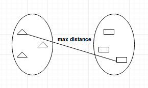
- Complete-linkage: calculates the maximum distance between clusters before merging.
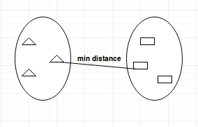
- Single-linkage: calculates the minimum distance between the clusters before merging. This linkage may be used to detect high values in your dataset which may be outliers as they will be merged at the end.
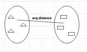
- Average-linkage: calculates the average distance between clusters before merging.
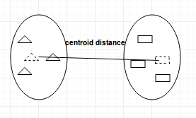
- Centroid-linkage: finds centroid of cluster 1 and centroid of cluster 2, and then calculates the distance between the two before merging.
The choice of linkage method entirely depends on you and there is no hard and fast method that will always give you good results. Different linkage methods lead to different clusters.
Dendrograms
In hierarchical clustering, you categorize the objects into a hierarchy similar to a tree-like diagram which is called a dendrogram. The distance of split or merge (called height) is shown on the y-axis of the dendrogram below.
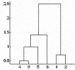
In the above figure, at first 4 and 6 are combined into one cluster, say cluster 1, since they were the closest in distance followed by points 1 and 2, say cluster 2. After that 5 was merged in the same cluster 1 followed by 3 resulting in two clusters. At last the two clusters are merged into a single cluster and this is where the clustering process stops.
One question that might have intrigued you by now is how do you decide when to stop merging the clusters? Well, that depends on the domain knowledge you have about the data. For, example if you are clustering football players on a field based on their positions on the field which will represent their coordinates for distance calculation, you already know that you should end with only 2 clusters as there can be only two teams playing a football match.
But sometimes you don't have that information too. In such cases, you can leverage the results from the dendrogram to approximate the number of clusters. You cut the dendrogram tree with a horizontal line at a height where the line can traverse the maximum distance up and down without intersecting the merging point. In the above case it would be between heights 1.5 and 2.5 as shown:
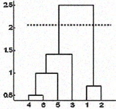
If you make the cut as shown you will end up with only two clusters.
Note that it is not necessary to make a cut only at such places, you can choose any point as the cut point depending on how many clusters you want. For example, the cut below 1.5 and above 1 will give you 3 clusters.
Note this is not a hard and fast rule to decide number of clusters. You can also consider plots like Silhouette plot, elbow plot, or some numerical measures such as Dunn's index, Hubert's gamma, etc.. which shows the variation of error with the number of clusters (k), and you choose the value of k where the error is smallest.
Measuring the goodness of Clusters
Perhaps the most important part in any unsupervised learning task is the analysis of the results. After you have performed the clustering using any algorithm and any sets of parameters you need to make sure that you did it right. But how do you determine that?
Well, there are many measures to do this, perhaps the most popular one is the Dunn's Index. Dunn's index is the ratio between the minimum inter-cluster distances to the maximum intra-cluster diameter. The diameter of a cluster is the distance between its two furthermost points. In order to have well separated and compact clusters you should aim for a higher Dunn's index.
Hierarchical Clustering in Action
Now you will apply the knowledge you have gained to solve a real world problem.
You will apply hierarchical clustering on the seeds dataset. This dataset consists of measurements of geometrical properties of kernels belonging to three different varieties of wheat: Kama, Rosa and Canadian. It has variables which describe the properties of seeds like area, perimeter, asymmetry coefficient etc. There are 70 observations for each variety of wheat. You can find the details about the dataset here.
Start by importing the dataset into a dataframe with the read.csv() function.
Note that the file doesn't have any headers and is tab-separated. To maintain reproducibility of the results you need to use the set.seed() function.
set.seed(786)
file_loc <- 'seeds.txt'
seeds_df <- read.csv(file_loc,sep = '\t',header = FALSE)
Since the dataset doesn't have any column names you will give columns name yourself from the data description.
feature_name <- c('area','perimeter','compactness','length.of.kernel','width.of.kernal','asymmetry.coefficient','length.of.kernel.groove','type.of.seed')
colnames(seeds_df) <- feature_name
It's advisable to gather some basic useful information about the dataset like its dimensions, data types and distribution, number of NAs etc. You will do so by using the str(), summary() and is.na() functions in R.
str(seeds_df)
summary(seeds_df)
any(is.na(seeds_df))
Note that this dataset has all the columns as numerical values. There are no missing values in this dataset that you need to clean before clustering. But the scales of the features are different and you need to normalize it. Also, the data is labeled and you already have the information about which observation belongs to which variety of wheat.
You will now store the labels in a separate variable and exclude the type.of.seed column from your dataset in order to do clustering. Later you will use the true labels to check how good your clustering turned out to be.
seeds_label <- seeds_df$type.of.seed
seeds_df$type.of.seed <- NULL
str(seeds_df)
As you will notice you have dropped the true label column from your dataset.
Now you will use R's scale() function to scale all your column values.
seeds_df_sc <- as.data.frame(scale(seeds_df))
summary(seeds_df_sc)
Notice the mean of all the columns is 0 and the standard deviation is 1. Now that you have pre-processed your data it's time to build the distance matrix. Since all the values here are continuous numerical values, you will use the euclidean distance method.
dist_mat <- dist(seeds_df_sc, method = 'euclidean')At this point you should decide which linkage method you want to use and proceed to do hierarchical clustering. You can try all kinds of linkage methods and later decide on which one performed better. Here you will proceed with average linkage method.
You will build your dendrogram by plotting the hierarchical cluster object which you will build with hclust(). You can specify the linkage method via the method argument.
hclust_avg <- hclust(dist_mat, method = 'average')
plot(hclust_avg)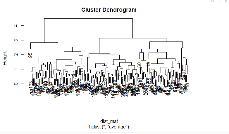
Notice how the dendrogram is built and every data point finally merges into a single cluster with the height(distance) shown on the y-axis.
Next, you can cut the dendrogram in order to create the desired number of clusters. Since in this case you already know that there could be only three types of wheat you will choose the number of clusters to be k = 3, or as you can see in the dendrogram h = 3 you get three clusters. You will use R's cutree() function to cut the tree with hclust_avg as one parameter and the other parameter as h = 3 or k = 3.
cut_avg <- cutree(hclust_avg, k = 3)If you visually want to see the clusters on the dendrogram you can use R's abline() function to draw the cut line and superimpose rectangular compartments for each cluster on the tree with the rect.hclust() function as shown in the following code:
plot(hclust_avg)
rect.hclust(hclust_avg , k = 3, border = 2:6)
abline(h = 3, col = 'red')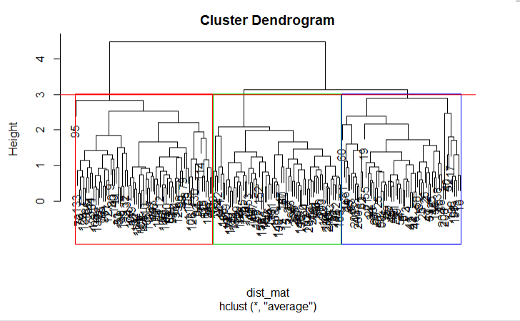
Now you can see the three clusters enclosed in three different colored boxes. You can also use the color_branches() function from the dendextend library to visualize your tree with different colored branches.
Remember that you can install a package in R by using the install.packages('package_name', dependencies = TRUE) command.
suppressPackageStartupMessages(library(dendextend))
avg_dend_obj <- as.dendrogram(hclust_avg)
avg_col_dend <- color_branches(avg_dend_obj, h = 3)
plot(avg_col_dend)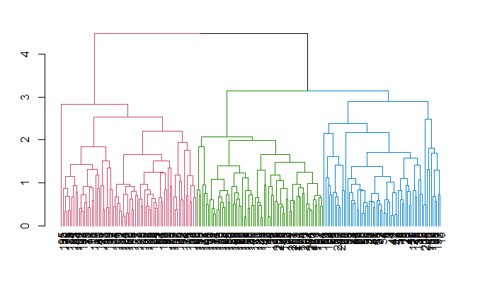
Now you will append the cluster results obtained back in the original dataframe under column name the cluster with mutate(), from the dplyr package and count how many observations were assigned to each cluster with the count() function.
suppressPackageStartupMessages(library(dplyr))
seeds_df_cl <- mutate(seeds_df, cluster = cut_avg)
count(seeds_df_cl,cluster)
You will be able to see how many observations were assigned in each cluster. Note that in reality from the labeled data you had 70 observations for each variety of wheat.
It's common to evaluate the trend between two features based on the clustering that you did in order to extract more useful insights from the data cluster-wise. As an exercise, you can analyze the trend between wheat's perimeter and area cluster-wise with the help of ggplot2 package.
suppressPackageStartupMessages(library(ggplot2))
ggplot(seeds_df_cl, aes(x=area, y = perimeter, color = factor(cluster))) + geom_point()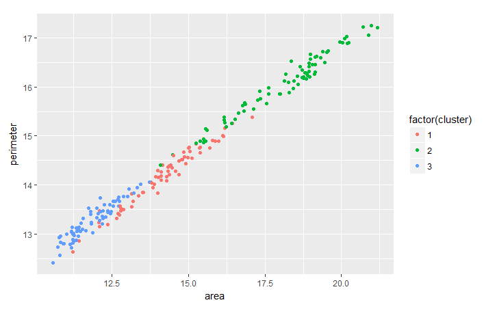
Notice that for all the varieties of wheat there seems to be a linear relationship between their perimeter and area.
Since you already have the true labels for this dataset, you can also consider cross-checking your clustering results using the table() function.
table(seeds_df_cl$cluster,seeds_label)If you have a look at the table that got generated, you clearly see three groups with 55 elements or more. Overall, you can say that your clusters adequately represent the different types of seeds because originally you had 70 observations for each variety of wheat. The larger groups represent the correspondence between the clusters and the actual types.
Note that in many cases you don't actually have the true labels. In those cases, as already discussed, you can go for other measures like maximizing Dunn's index. You can calculate dunn's index by using the dunn() function from the clValid library. Also, you can consider doing cross validation of the results by making train and test sets, just like you do in any other machine learning algorithm, and then doing the clustering when you do have the true labels.
Comparing with K-Means Clustering Algorithm
You might have heard about the k-means clustering algorithm; if not, take a look at this tutorial. There are many fundamental differences between the two algorithms, although any one can perform better than the other in different cases. Some of the differences are:
- Distance used: Hierarchical clustering can virtually handle any distance metric while k-means rely on euclidean distances.
- Stability of results: k-means requires a random step at its initialization that may yield different results if the process is re-run. That wouldn't be the case in hierarchical clustering.
- Number of Clusters: While you can use elbow plots, Silhouette plot etc. to figure the right number of clusters in k-means, hierarchical too can use all of those but with the added benefit of leveraging the dendrogram for the same.
- Computation Complexity: K-means is less computationally expensive than hierarchical clustering and can be run on large datasets within a reasonable time frame, which is the main reason k-means is more popular.
Conclusion
Congrats! You have made it to the end of this tutorial. You learned how to pre-process your data, the basics of hierarchical clustering and the distance metrics and linkage methods it works on along with its usage in R. You also know how hierarchical clustering differs from the k-means algorithm. Well done! But there's always much more to learn. I suggest you take a look at our Unsupervised Learning in R course.


