Markov Chain Monte Carlo (MCMC): Sample Complex Probability Distributions

Some probability distributions are just too complex for you to directly work with.

When you're modeling real-world data, the math often breaks down before you get anywhere useful. It often happens that integrals look manageable on paper, but turn intractable the moment you add a couple of latent variables. This is especially common in Bayesian inference, where the posterior distribution combines your prior beliefs with observed data - and the result is something you can't summarize with a simple formula.

The basic idea of Markov Chain Monte Carlo is that instead of directly working on the math, MCMC explores the distribution through simulation. It draws samples that reflect its shape without ever needing to compute it in full.

In this article, I'll cover the core concepts behind MCMC, walk through the most common algorithms, and show you how to put it to work in Python.

Do you need a Python math refresher? Read our Demystifying Mathematical Concepts for Deep Learning blog posts to see math applied in Numpy.

What Is Markov Chain Monte Carlo?

Markov Chain Monte Carlo (MCMC) is a family of algorithms that generate samples from probability distributions - even when those distributions are too complex to directly work with.

The name breaks into two parts. The Markov chain controls how the algorithm moves through possible states. Each step depends only on where you are right now, not on the full history of how you got there. The Monte Carlo part means you're using random sampling to estimate quantities of interest.

Combined, MCMC builds a chain of random samples that, over time, reflects the shape of your target distribution. It's a sampling technique first and foremost. You're not solving the math exactly, just approximating it through simulation.

Why Markov Chain Monte Carlo Is Needed

The problem with real-world data distribution is they aren’t nearly as clean as the textbook ones.

In Bayesian inference, you're often trying to compute a posterior distribution - the updated probability of your model parameters after seeing data. The formula looks easy on paper: just multiply the prior by the likelihood, then divide by the marginal likelihood. That last term requires integrating over every possible parameter value. In high dimensions, that integral is practically impossible to compute.

It only gets worse as your model grows. When you add more parameters or more latent variables, the exact computation becomes a dead end. You'll run into this across a range of common scenarios:

• Bayesian hierarchical models: Where parameters depend on other parameters, creating nested distributions that don't cleanly integrate
• High-dimensional posteriors: Where the number of parameters makes grid-based approximations computationally infeasible
• Non-conjugate priors: Where the prior and likelihood don't combine into a recognizable distribution

MCMC is a good workaround in these scenarios. Instead of computing the distribution, it draws samples from it. Those samples have everything you need without ever solving the integral.

The Two Ideas Behind MCMC

MCMC combines two ideas that are simple enough on their own, but powerful when combined. Let me walk you through them.

Markov chains

A Markov chain is a sequence of states where each step depends only on where you are right now.

Where you've been before doesn't matter. Only your current state determines where you go next. This "memoryless" property - formally called the Markov property - is what makes the math easy to manage and the algorithm practical.

The chain moves through states one step at a time, and with the right setup, it eventually settles into a stationary distribution - a stable pattern where the probability of being in any given state stops changing. That stable distribution is exactly what MCMC is designed to work with.

Monte Carlo methods

Monte Carlo methods use random sampling to estimate quantities that are hard to directly compute.

The idea is to draw enough random samples from a distribution, and then estimate its mean, variance, or any other property just by looking at the samples. The more samples you draw, the closer your estimates get to the true values.

On their own, Monte Carlo methods require you to directly sample from the distribution - which is exactly the problem we're trying to solve. Markov chains handle that part.

How Markov Chain Monte Carlo Works

MCMC is a loop with a simple decision at each step.

1. Start with an initial state: Pick a starting point in your parameter space, even if it's a rough guess
2. Propose a new state: Use a proposal mechanism to suggest where to move next
3. Decide whether to accept it: Compare the proposed state to the current one and accept or reject based on how probable each is under the target distribution
4. Repeat: Run this loop thousands of times, collecting samples along the way
5. Use the samples: Estimate means, credible intervals, or any other quantity of interest from the collected samples

The accept/reject step is where the “magic” happens.

By accepting better states more often than worse ones, the chain gravitates toward regions of high probability - without ever needing to compute the full distribution.

Early samples depend on where you started, so those get discarded. After enough iterations, the chain forgets its starting point and the remaining samples reflect the true shape of your target distribution.

The Target Distribution and Stationary Distribution

MCMC is built around a goal of generating samples from a target distribution you can't sample from directly.

The target distribution is whatever you're trying to learn about - usually a posterior distribution in Bayesian inference. You know its shape up to a normalizing constant, but you can't directly compute that constant. MCMC doesn't need it.

Every MCMC algorithm is designed so that its Markov chain has a stationary distribution that matches the target. A stationary distribution is the distribution the chain settles into after enough steps.

Keep the chain running and it'll start producing samples that look just like draws from your target distribution. The integral gets bypassed.

Popular Markov Chain Monte Carlo Algorithms

There are a handful of MCMC algorithms you'll see in practice. They all follow the same core loop, but differ in how they propose new states and how they use information about the target distribution.

Metropolis algorithm

The Metropolis algorithm is the simplest MCMC algorithm and the one that started it all.

At each step, it proposes a new state by adding random noise to the current one. If the proposed state has higher probability under the target distribution, it's always accepted. If it's lower, it's accepted with a probability proportional to the ratio of the two probabilities - otherwise, the chain stays put.

This accept/reject mechanism means the chain will spend more time in high-probability regions without ever computing the full distribution.

The Metropolis algorithm uses a symmetric proposal distribution, meaning it’s equally likely to propose a step in any direction. It tends to break down as models grow.

Metropolis-Hastings algorithm

The Metropolis-Hastings (MH) algorithm generalizes Metropolis by allowing asymmetric proposal distributions.

MH adjusts the acceptance probability to account for the fact that some proposals are more likely than others. You can tune the proposal to the shape of your target, which leads to better exploration and faster convergence.

Most modern MCMC methods are extensions of MH or built on the same principles. So if you understand Metropolis-Hastings, you’ll understand the foundation of the field.

Gibbs sampling

Gibbs sampling updates one variable at a time instead of proposing a new state for all parameters at once.

At each step, it samples each variable from its conditional distribution - the distribution of that variable given the current values of all the others. When you’ve cycled through all variables, you've completed one full iteration.

This entirely avoids the accept/reject step, since each conditional draw is always accepted. It's handy when the full joint distribution is hard to sample from but the conditionals are tractable, which is common in Bayesian hierarchical models.

Hamiltonian Monte Carlo

Hamiltonian Monte Carlo (HMC) is the first algorithm that made modern Bayesian inference practical at scale.

Instead of randomly proposing new states, HMC uses gradient information from the target distribution to propose states that are far from the current position but still likely to be accepted. It moves through the parameter space far better than random-walk methods. There are fewer rejected proposals and better exploration of high-dimensional distributions.

Random-walk methods like Metropolis don’t scale as the number of parameters grows. HMC doesn't have that problem to the same degree.

HMC is the engine behind Stan, one of the most widely used probabilistic programming platforms. The No-U-Turn Sampler (NUTS), which is an adaptive extension of HMC used in PyMC, removes the need to manually tune step size and number of steps.

Markov Chain Monte Carlo in Bayesian Statistics

If there's one area where MCMC has had the biggest impact, it's Bayesian inference.

Bayesian statistics centers on the posterior distribution, which is the updated probability of your model parameters after seeing data. Computing it means multiplying the prior by the likelihood and normalize. That normalization step requires an integral that's rarely tractable.

MCMC entirely removes this step. You just evaluate the unnormalized posterior at any given point and let the chain do the rest.

Here's a simple example. Say you're estimating the bias of a coin. You start with a prior belief that the coin is probably fair, then observe a sequence of flips. For a simple coin model, the posterior has a closed form. If you add a hierarchical structure, meaning estimating bias across a hundred coins simultaneously, it becomes impossible to compute.

With MCMC, you run the chain, collect samples from the posterior, and use those samples to compute what you need.

Understanding Burn-In, Convergence, and Mixing

These three concepts confuse data scientists new to MCMC. If you get them wrong, you’ll get the results, but you won’t know why they’re unreliable.

Burn-in

When a Markov chain starts, it has no idea where the high-probability regions of your target distribution are.

Those early samples are influenced by your starting point, not by the target distribution. Burn-in is the practice of discarding them. You run the chain for some number of iterations first, throw those samples away, and only keep what comes after the chain has had time to find a good starting point.

There's no universal rule for how long burn-in should be. It depends on your model, your starting point, and how well the chain mixes. In practice, you diagnose it visually with trace plots rather than picking a fixed number upfront.

Convergence

Convergence means the chain has stopped being influenced by its starting point and is now drawing samples that reflect the target distribution.

A chain that hasn't converged produces biased samples. The mean you compute from them won't match the true posterior mean. Instead, it'll reflect wherever the chain happened to be stuck.

Convergence is something you assess after the fact using diagnostics. Running multiple chains from different starting points and checking whether they agree is one of the most reliable ways to catch convergence failures.

Mixing

A chain that converges but mixes poorly is still problematic.

Mixing describes how well the chain explores the target distribution. A well-mixing chain moves around freely, visiting both high and low-probability regions and producing samples that are roughly independent of each other. A poorly mixing chain stays in one region for many iterations before moving, and produces highly correlated samples that don't represent the full distribution.

Poor mixing often shows up as a trace plot that looks like a slow, meandering river instead of a noisy horizontal band. When you see that, your sampler needs tuning - a better proposal distribution or a different algorithm altogether.

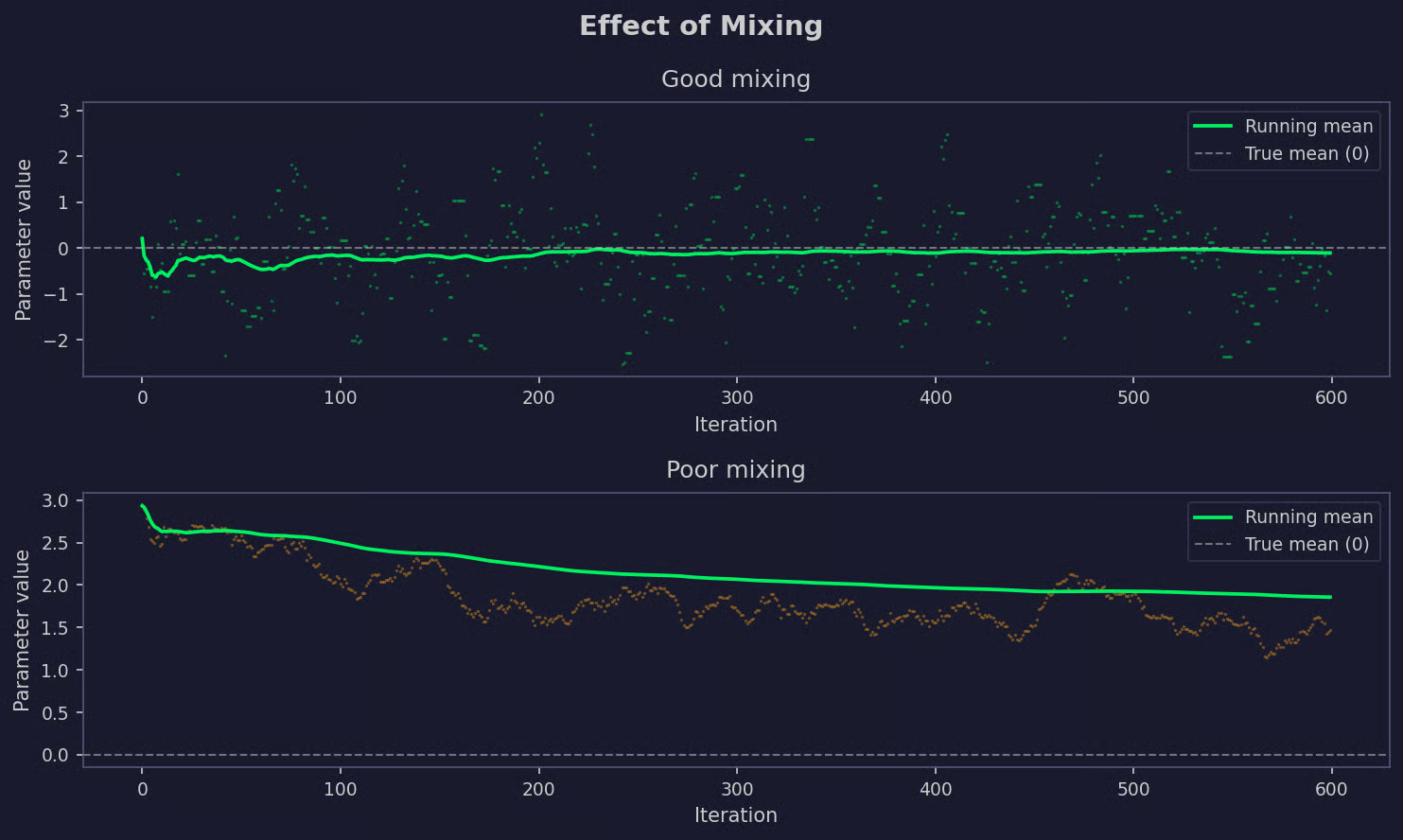
Mixing comparison plot

How to Evaluate MCMC Results

I’ll now show you four ways you can evaluate MCMC and explain when to use each.

Trace plots

A trace plot shows the sampled value of a parameter at each iteration. It's the first thing you should look at after running MCMC.

A healthy trace plot looks like white noise around a stable mean. You shouldn’t see trends, long flat stretches, or slow drift. If you see the chain wandering or getting stuck in one region for many iterations, that's a mixing problem and your samples aren't reliable.

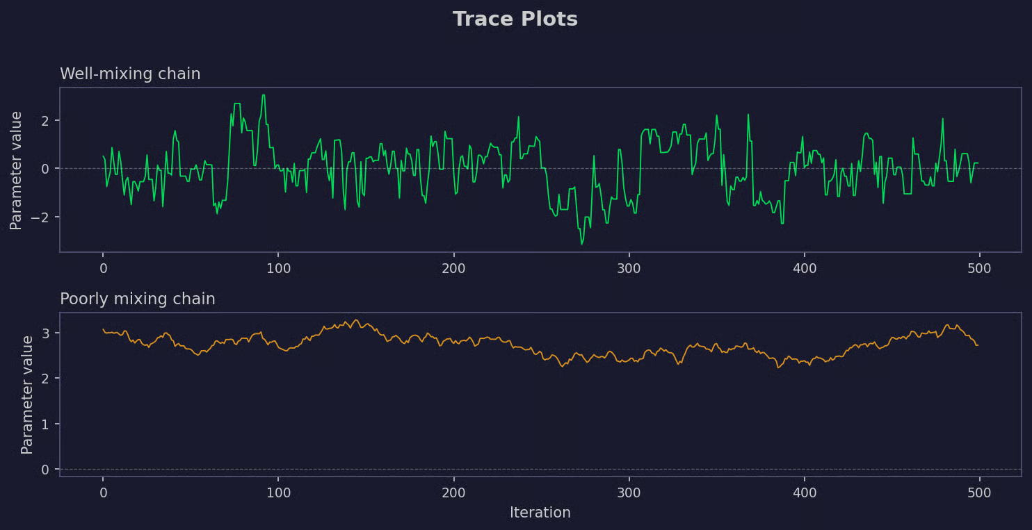
Trace plots visualized

Autocorrelation

MCMC samples are never fully independent. Each sample is influenced by the one before it. Autocorrelation measures how strongly samples are correlated across iterations.

High autocorrelation means your samples carry less information than their count suggests. Two thousand correlated samples might give you the same information as two hundred independent ones. Most MCMC libraries include autocorrelation plots so you can see how quickly the correlation drops off as samples get further apart.

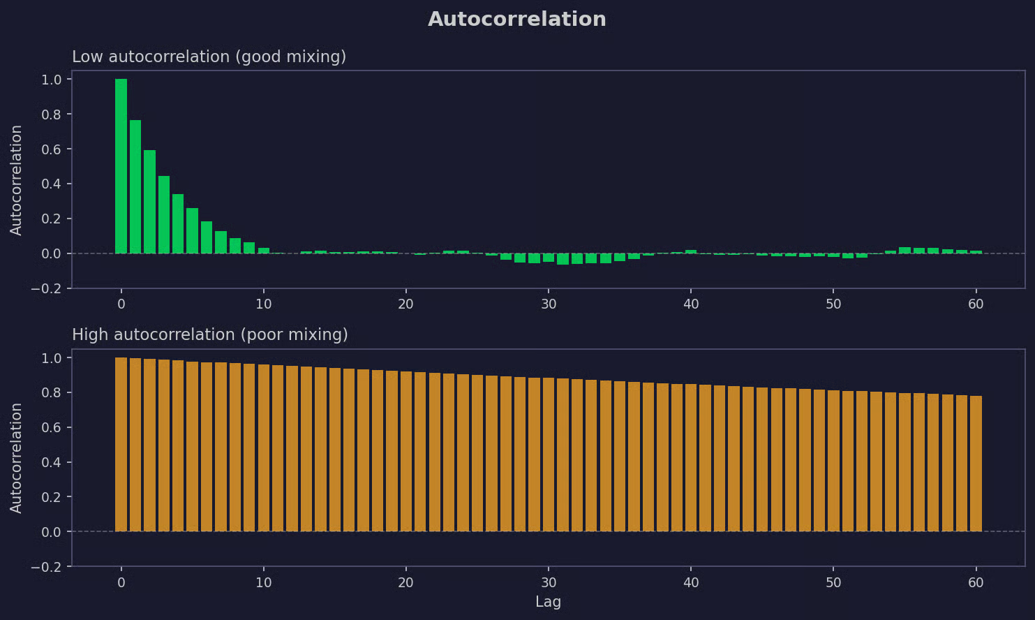
Autocorrelation plots visualized

Effective sample size

Effective sample size (ESS) translates that autocorrelation into a practical number: how many independent samples your chain is equivalent to.

If you drew 5,000 samples but the ESS is 200, you're working with the statistical power of 200 independent draws. A low ESS means you need to run your chain longer, tune the sampler, or both. Most practitioners aim for an ESS of at least a few hundred per parameter before trusting their estimates.

Convergence diagnostics

When you run multiple chains, you can formally test whether they've converged to the same distribution. The Gelman-Rubin diagnostic, reported as R-hat, compares variance within each chain to variance across chains.

An R-hat close to 1.0 means the chains agree, which is a good sign. Values above 1.01 or 1.05 (depending on the threshold your library uses) suggest the chains haven't converged and you need more iterations. Most modern libraries like PyMC automatically compute R-hat and flag warnings when it's too high.

Markov Chain Monte Carlo in Python

Python has a couple of libraries for MCMC, each with a different philosophy.

• PyMC: The most approachable option for most data scientists. You define your model using Python syntax, and PyMC handles the sampling under the hood using NUTS (an adaptive version of HMC). It's the go-to for Bayesian modeling in Python.
• CmdStanPy / PyStan: Python interfaces to Stan, a dedicated probabilistic programming language. Stan compiles your model to C++ before running it, which makes it fast and well-suited for complex hierarchical models. The tradeoff is a steeper learning curve.
• NumPy: No dedicated MCMC library, but you can implement algorithms like Metropolis-Hastings from scratch. Useful for understanding what's happening under the hood before moving to higher-level tools.

For most practical work, PyMC is where you'd start. This is what I’ll use, so if you’re following along, make sure to install the library first:

pip install pymc

To keep things simple, I’ll stick to an easy example, which is estimating the bias of a coin from a sequence of flips.

Step 1: Define the model

import pymc as pm
import numpy as np

# 1 = heads, 0 = tails
observed_flips = np.array([1, 0, 1, 1, 0, 1, 1, 1, 0, 1])

with pm.Model() as coin_model:
    # Prior: we believe the coin is probably fair
    bias = pm.Beta("bias", alpha=2, beta=2)

    # Likelihood: observed flips given the bias
    flips = pm.Bernoulli("flips", p=bias, observed=observed_flips)

The pm.Beta prior encodes a weak belief that the coin is fair. The pm.Bernoulli likelihood connects the model to the observed data.

Step 2: Run the sampler

with coin_model:
    trace = pm.sample(2000, tune=1000, return_inferencedata=True)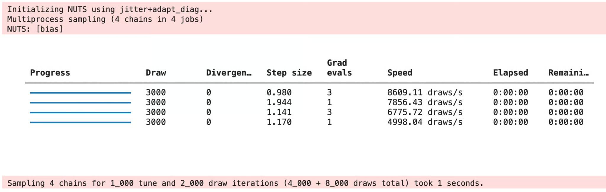

Output of running the sampler

tune sets the number of burn-in steps - those samples get discarded. sample draws 2000 posterior samples per chain after tuning.

Step 3: Inspect the posterior

import arviz as az

az.plot_trace(trace, var_names=["bias"])
az.summary(trace, var_names=["bias"])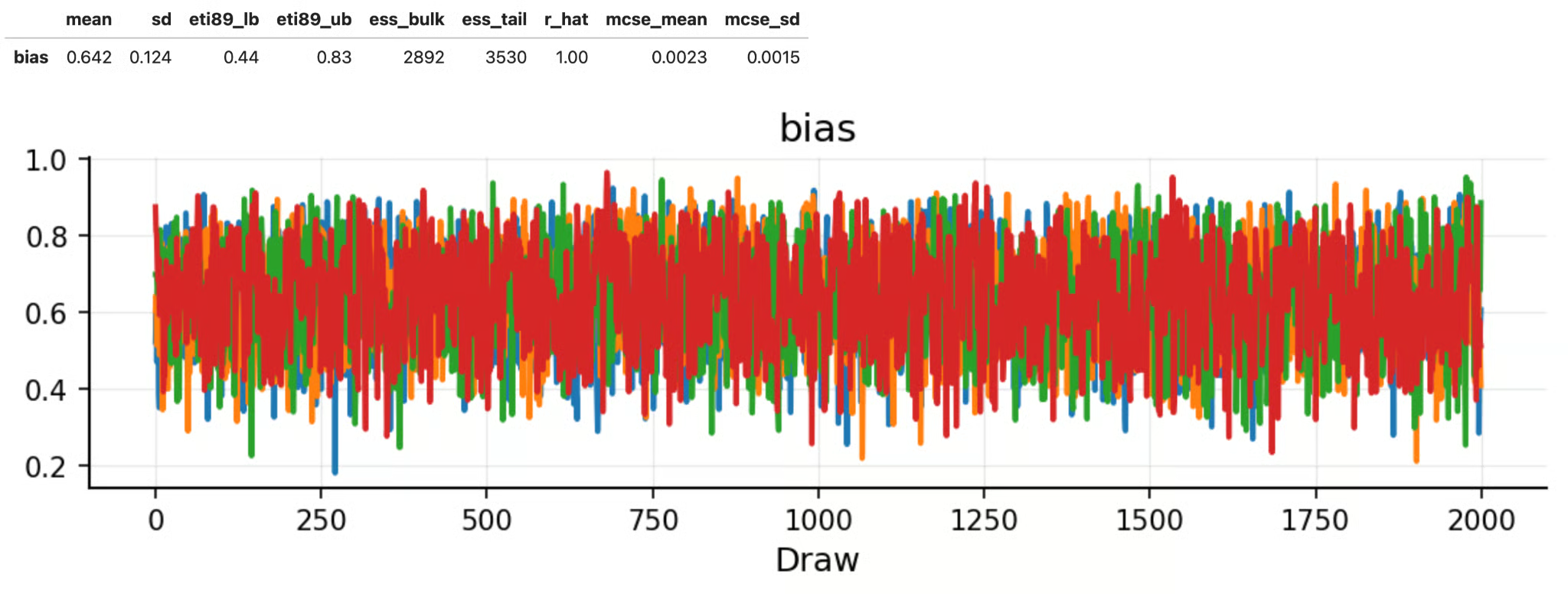

Model trace plot and summary results

az.summary() gives you the posterior mean, standard deviation, and R-hat for each parameter. If R-hat is close to 1.0, the chains have converged. az.plot_trace() plots the trace and posterior distribution side by side for each parameter.

For this dataset - 7 heads out of 10 flips - the posterior mean equals 0.642 with a standard deviation of 0.124. This reflects the evidence in the data while staying close to the fair-coin prior. R-hat is 1.00 and ESS is well above 2000, so the chains have converged and the samples are reliable.

Common Mistakes with MCMC

MCMC is easy to run, but it’s also easy to misuse. Here are the mistakes that show up most often.

• Assuming convergence too early: Just because the sampler ran without errors doesn't mean it converged. Always check R-hat and trace plots before trusting your results. A chain can look stable and still be stuck in one region of the parameter space.
• Ignoring burn-in: Early samples are biased toward your starting point, not your target distribution. Discard them. Most libraries handle this automatically via the tune parameter, but check that you're not accidentally including those samples in your analysis.
• Poor mixing: A chain that moves too slowly produces highly correlated samples that carry less information than their count suggests. If your trace plot looks like a slow drift rather than noisy horizontal band, your proposal distribution needs tuning, or you need a better algorithm. Switching from Metropolis to NUTS often fixes this outright.
• Too few samples: A low effective sample size (ESS) means your estimates are unreliable, even if the chain technically converged. If your ESS is a small fraction of your total draws, run the chain longer or improve mixing before drawing conclusions.

MCMC vs Other Sampling Methods

MCMC isn't the only way to approximate a distribution. Here's how it compares to the alternatives.

• Rejection sampling draws proposals from a simpler distribution and accepts them based on how well they match the target. It's exact when it works, but acceptance rates collapse in high dimensions.
• Importance sampling weights samples from a proposal distribution to approximate expectations under the target. It's fast and works well in low dimensions, but the variance of the weights explodes as dimensionality increases. In practice, a handful of samples end up carrying almost all the weight, which makes estimates unreliable.
• Variational inference (VI) fits a simpler distribution to approximate the target by minimizing a divergence measure. VI is much faster than MCMC and scales to large datasets, but it introduces approximation error. The fitted distribution may miss posterior structure that MCMC would catch.

Here's the short version:

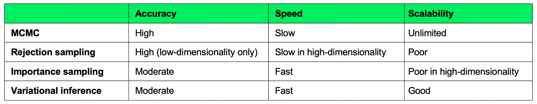
MCMC versus alternatives

MCMC is the right choice when accuracy matters more than speed. If you need to scale to large datasets or run inference in real time, variational inference could be worth the accuracy tradeoff.

Conclusion

MCMC is one of those tools that looks intimidating from the outside but makes a lot of sense once you understand what it's actually doing - building a chain of samples that gradually reflects the shape of a distribution you can't compute directly.

It’s also a lot easier to comprehend when you break it into parts: Markov Chains and Monte Carlo methods.

Its role in Bayesian statistics is hard to overstate. Posterior distributions that would otherwise be out of reach become solvable the moment you have a reliable sampler. That's why MCMC is at the core of probabilistic programming libraries like PyMC and Stan.

But before jumping into implementation, you should get the intuition right. Understand why the chain needs to burn in, what mixing actually means, and how to read a trace plot. The code itself is the easy part, as Python libraries hide all the abstractions behind simple function calls.

If you want to become proficient in machine learning, enroll in our Machine Learning Scientist in Python track. 85 hours of materials will help you get job-ready in 2026.