Introduction
Two major classes of numerical problems that arise in data analysis procedures are optimization and integration problems. It is not always possible to analytically compute the estimators associated with a given model, and we are often led to consider numerical solutions. One way to avoid that problem is to use simulation. Monte Carlo estimation refers to simulating hypothetical draws from a probability distribution, in order to calculate significant quantities of that distribution.
The basic idea of Monte Carlo consist of writing the integral as an expected value with respect to some probability distribution, and then approximated using the method of moment estimator ($E[g(X)] \approx \overline{g(X)} = \dfrac{1}{n}\sum g(X_{i})$).
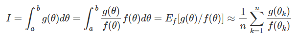
If we have a continuous function $g(\theta)$ and we want to integrated in the interval (a,b), we can rewrite our integral as an expected value of an uniform distribution $U \sim U[a,b]$, that is:
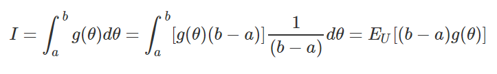
Using the method of moments estimator our integral approximation is:
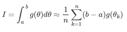
Where the
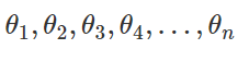
Are simulated values from a uniform distribution.
Example 1: Exponential integral approximation
1) Given a function $f(x)= e^{x}$ the integral in the interval [3,5] is:
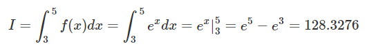
The MonteCarlo approximation of the integral is:
#       Declaring the desired function
f = function(x){return(exp(x))}
#       Declaring the absolute error function
error = function(x,y){return(abs(x-y))}
#       The actual integral answer
ans = exp(5)-exp(3)

set.seed(6971)
#       number of iterations
n = 10^2
#       simulated uniform data
x= runif(n,3,5)
#       MonteCarlo approximation
MCa= (5-3)*mean(f(x))
#       Approximation error
e = error(ans,MCa)

rest =  data.frame(n = n,MCapprox = MCa,error = e)
set.seed(6971)
for(k in 3:6){
  n = 10^k
  x = runif(n,3,5)
  mca = (5-3)*mean(f(x))
  rest = rbind(rest,c(n,mca,error(ans,mca) ) )
}

kable(rest,digits = 5,align = 'c',caption = "Integral Monte Carlo approximation results",
      col.names =c("Number of simulations","Monte Carlo approximation","Error approximation"))
Generalized Monte Carlo Approximation
In a general case, the integral approximation for a given distribution f is:
An algorithm for construction of $\widehat{I}$ can be described by the following steps:
1) Generate ![]() from a f distribution
from a f distribution
2) Calculate: ![]()
3) Obtain the sample mean: $$\overline{I} = \dfrac{1}{n}\sum_{k=1}^{n}\dfrac{g(\theta_k)}{f(\theta_k)}$$
In the next chunk, the simple Monte Carlo approximation function is presented to show how the algorithm works, where a and b are the uniform density parameters, n the number of desired simulations, and f is the function that we want to integrate.
# The simple Monte Carlo function
MCaf = function(n,a,b,f){
x = runif(n,a,b)
MCa = (b-a)*mean(f(x))
return(MCa)
}
Monte Carlo Methods in Bayesian Data Analysis
The main idea of the Bayesian data analysis is fitting a model ( such as a regression or a time series model ) using a Bayesian inference approach. We assume that our parameters of interest have a theoretical distribution, this distribution (posterior) is updated using the distribution of the observed data (likelihood), and the previous or external information about our parameters (prior distribution) by using the Bayes' theorem.
$$p(\theta / X) \text{ } \alpha\text{ } p(X/\theta)p(\theta)$$ Where:
$p(\theta/X)$ is the parameter posterior distribution
$p(X/\theta)$ is the sampling distribution of the observed data ( likelihood ).
$p(\theta)$ is the parameter prior distribution.
The main problem in the Bayesian approach is estimating the posterior distribution. The Markov Chain Monte Carlo methods ( mcmc ) generate a sample of the posterior distribution and approximate the expected values, probabilities or quantiles using Monte Carlo methods.
In the next two sections, we provide two examples for approximating probabilities and quantiles of a theoretical distribution. The procedure presented above are the usual methodologies used in a Bayesian approach.
Example 2: Probability approximation of a gamma distribution
Lets suppose we want to calculate the probability that a random variable $\theta$ is between zero and 5 $P(0 < \theta < 5)$, where $\theta$ has gamma distribution with parameter a = 2 and b = 1/3 ($\theta \sim Gamma(a = 2,b = 1/3)$), so the probability is:

Where $I_{[0,5]}(\theta) = 1$ if $\theta$ belongs to the interval [0,5].The idea of the Monte Carlo approximation, is count the number of observations that belong to the interval [0,5], and divide it by the total of the simulated data.
set.seed(6972)
#       number of iterations
n = 10^2
#       simulated uniform data
x= rgamma(n,shape = 2,1/3)
#       MonteCarlo approximation
MCa= mean(x <= 5)
#       Approximation error
e = error(pgamma(5,2,1/3),MCa)

rest =  data.frame(n = n,MCapprox = MCa,error = e)

for(k in 3:6){
  n = 10^k
  x= rgamma(n,shape = 2,1/3)
  mca= mean(x <= 5)
 rest = rbind(rest,c(n,mca,error(pgamma(5,2,1/3),mca) ) )
}

kable(rest,digits = 5,align = 'c',caption = "Probability Monte Carlo approximation results",
      col.names =c("Number of simulations","Monte Carlo approximation","Error approximation"))
Example 3: Quantile approximation of a normal distribution
Lets suppose we want to calculate the 0.95 quantile of a random variable $\theta$ that has normal distribution with parameters $\mu = 20$ and $\sigma = 3$ ($\theta \sim normal(\mu = 20,\sigma^{2} = 9)$), so the 0.95 quantile is:
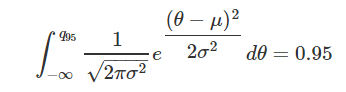
The main idea is found the largest sample value that gives a probabilty equal or less than 0.95, the Monte Carlo quantile approximation is estimate it using the quantile() function of the simulated data.
set.seed(6973)
#       number of iterations
n = 10^2
#       simulated uniform data
  x= rnorm(n,20,3)
#       MonteCarlo approximation
MCa= quantile(x,0.95)
#       Approximation error
e = error(qnorm(0.95,20,3),MCa)

rest =  data.frame(n = n,MCapprox = MCa,error = e)

for(k in 3:6){
  n = 10^k
  x= rnorm(n,20,3)
  mca= quantile(x,0.95)
 rest = rbind(rest,c(n,mca,error(qnorm(0.95,20,3),mca) ) )
}

kable(rest,digits = 5,align = 'c',caption = "Quantile Monte Carlo approximation results",
      col.names =c("Number of simulations","Monte Carlo approximation","Error approximation"),row.names = FALSE)
Discussions and Conclusions
The Monte Carlo approximation methods offer an alternative tool for integral approximation and are a vital tool in the Bayesian inference approach, especially when we work with sophisticated and complex models. As it seems in all our three examples, the Monte Carlo methods offer an excellent approximation, but it demands a huge number of simulations for getting an approximation error close to zero.
References
1) Introducing Monte Carlo methods with R, Springer 2004, Christian P. Robert and George Casella.
2) Handbook of Markov Chain Monte Carlo, Chapman and Hall, Steve Brooks, Andrew Gelman, Galin L. Jones, and Xiao-Li Meng.
3) Introduction to mathematical Statistics, Pearson, Robert V. Hogg, Joseph W. Mckean, and Allen T. Craig.
4) Statistical Inference An Integrated Approach, Chapman and Hall, Helio S. Migon, Dani Gamerman, Francisco Louzada.