Discrete Probability Distributions Explained with Examples

Let me begin by asking you a question: What do the following scenarios all share in common? Counting website clicks, tracking defective products, and analyzing customer purchases. They all involve countable outcomes that form the foundation of discrete probability distributions.

Discrete probability distributions are tools which we can use for modeling situations where outcomes can be enumerated, such as 0, 1, 2, 3 customers, heads or tails, success or failure, etc. Unlike continuous distributions that handle measurable quantities like height or temperature, discrete distributions focus on countable events.

To give you some motivation, here are some examples of how these distributions are used in applications across industries:

• Netflix uses categorical distributions for recommendations
• Banks rely on binomial models for credit risk
• Manufacturers apply hypergeometric distributions in quality control sampling.

In this article, I will cover the theoretical foundations, practical applications, and hands-on examples you need to master discrete probability distributions. By the end, you will gain great conceptual understanding and practical skills for modeling real-world phenomena effectively.

What Is a Discrete Probability Distribution?

I have briefly mentioned what such a distribution is, but now I want to dive deep into it. At its core, a discrete probability distribution is just a way of assigning probabilities to a set of countable outcomes. The outcomes could be as simple as 0, 1, 2, 3… or they could be categories like “Red, Blue, Green.”

Formally speaking, if we have a discrete random variable X, the distribution is defined by a probability mass function (PMF). The PMF tells us the probability of each possible outcome p(x)=P(X=x).

There are, however, two key rules that must be followed in order for the distribution to be a valid discrete probability distribution:

1. p(x) >= 0 for all x
2. ∑p(x)=1 summed over all x

Let’s go through what this means. The first condition states that we need all probabilities of outcomes to be greater than or equal to 0, as a negative probability doesn’t make any sense! The second condition states that the sum of all event’s probabilities need to add up to 1. Now there are ways to make sure that this condition is met such as applying the softmax function to a distribution to make it into a valid probability distribution.

A classic example is rolling a fair six-sided die. Each face has a probability of 1/6, and if we sum all the probabilities (all six of them), we get 1.

Now you might have a question here:

Why is this important? 

It’s because discrete distributions give us a structured way to answer practical questions like:

• “What is the chance of getting 3 heads out of 5 flips?”
• “How many defective items should we expect in a batch?”
• “What is the likelihood that at least one customer buys today?”

Note that these aren’t abstract math problems I have just come up with! They connect directly to business metrics, risk models and product performance.

Discrete vs. Continuous Probability Distributions

At this point, you might have another question:

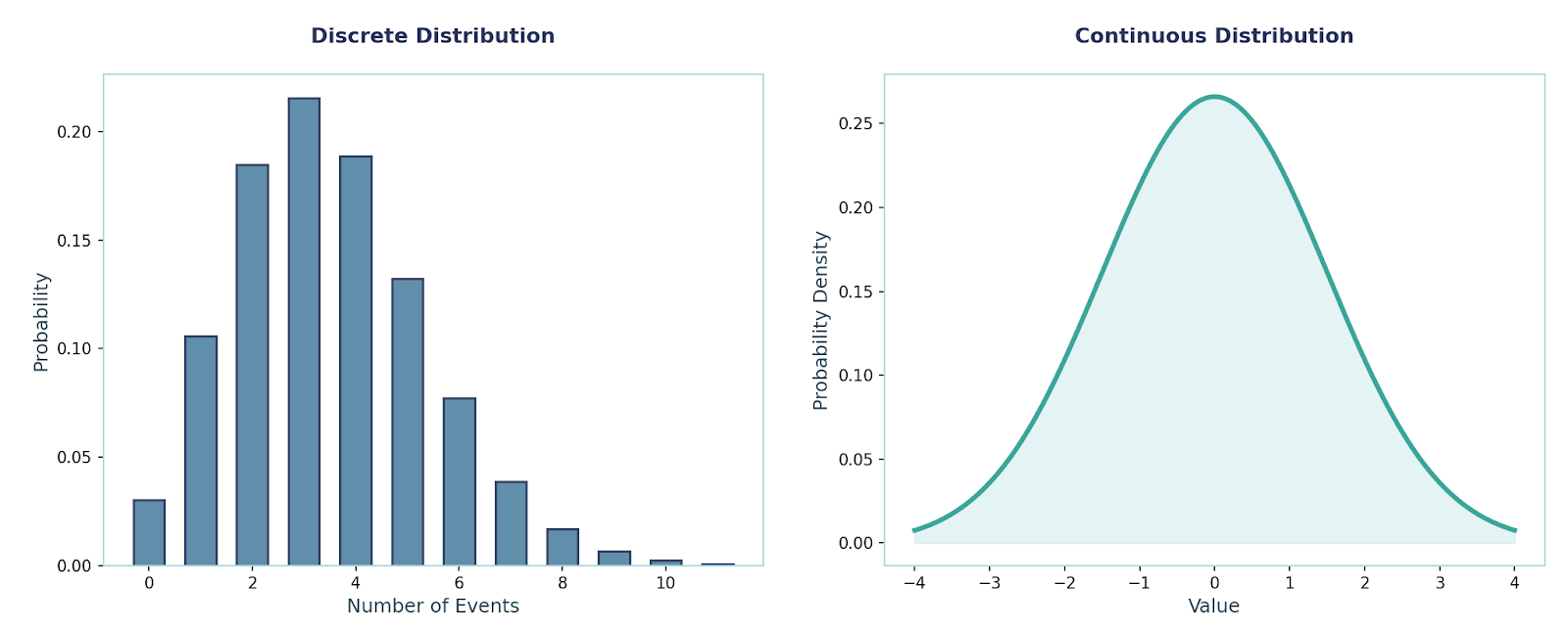
How do discrete distributions differ from continuous ones?

The short answer: discrete distributions handle counts, continuous distributions handle measurements.

• In discrete distributions, we talk about exact probabilities: P(X=2), meaning “what is the chance we see exactly two customers?”
• In continuous distributions, the probability of any exact point is zero (this is a very important point!). Instead, we talk about intervals such as P(160≤X≤170), meaning “what is the chance a person’s height falls between 160cm and 170cm?”

Here is another way to visualize this:

• Discrete distributions look like step functions. We can think of a bar chart where each bar is a probability for a count.
• Continuous distributions look like smooth curves. We can think of the bell curve for normal distributions.

A great follow-up question would be:

When to use which?

• Discrete: when the outcome is a count or a category, such as number of clicks, number of wins, defect vs. no defect, etc.
• Continuous: when the outcome is measured along a scale such as height, weight, temperature, time, etc.

Mathematical Foundations and Theoretical Framework

Before I formally introduce any of the Discrete Probability Distributions, I need to go over some mathematics that are important to fully understand each distribution.

Probability mass function (PMF)

The PMF tells us the probability of each exact value a discrete random variable X can take. 

Now the conditions that we covered before are what make a valid PMF:

1. p(x) >= 0 for all x
2. ∑p(x)=1 summed over all x

All in all, the PMF is quite useful for calculating things such as Mean, Variance and Moments. Let’s do a quick worked example together:

Let X∈{0,1,2,3}, with p(0)=0.1, p(1)=0.2, p(2)=0.3, p(3)=0.4. Let’s start off by finding the mean or the expected value. We can work it out mathematically using this:

E[X]=0*(0.1)+1*(0.2)+2*(0.3)+3*(0.4)=2.0This makes sense since we are taking every possible outcome’s value and multiplying it with its respective probability, giving us the Expected Value. Continuing on, we can work out the second moment E[X2]:

E[X^2]=0+1(0.2)+4(0.3)+9(0.4)=5.0

From this, we can work out the Varianc,e which can be calculated using this equation: Var(X) = E[X2] - (E[X])2

Therefore:

Var(X)=5.0−2.0^2=1.0

Cumulative distribution function (CDF)

Let’s now talk about the CDF, which is a function that adds up probabilities up to a threshold. For discrete probability distributions, it will be step functions due to its discretized nature. For clarity's sake, the CDF for a continuous distribution would have been a smooth continuous function (similar to a Sigmoid Function). 

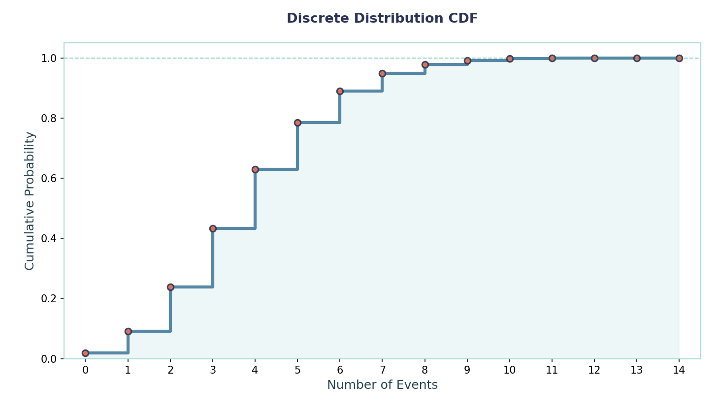
Mathematically, it is written as this: FX​(x)=P(X≤x)=∑{k<=x}​pX​(k). To make sure this is crystal clear, let’s do an example together: 

Suppose X can take values 0,1,2,3 with these respective probabilities:

• P(X=0)=0.1
• P(X=1)=0.2
• P(X=2)=0.3
• P(X=3)=0.4

To work out the CDF, all we have to do is create a threshold and add the respective probabilities whose outcome is within that threshold. For example, F(x < 3) =0.1 + 0.2 +0.3 = 0.6 (equivalently F(2) = 0.6). Obviously, for a continuous probability distribution, the CDF would be integration rather than summation.

Moments

Another piece of math which will be important is the MGF, but before that it is important to understand what a moment is. I have already mentioned moment before but now let’s dive deeper into this.

Moments are numbers that describe the shape of a probability distribution. They are like summaries that capture how the distribution is centered, how spread out it is, and even how lopsided or “peaked” it looks. The moments are first, second, third, etc. and they each tell you different things. 

For example, the first moment tells us about how the distribution is centered. This is also the same as the Expected Value which is also the same as the Mean.

Formally, the k-th moment about the origin is defined as E[Xk]=∑xk pX(x).

Let me give you some more information about some of the moments:

• 1st moment: E[X] → the mean, tells us the central location
• 2nd moment: E[X^2] → not variance yet, but related to how spread out things are
• 3rd moment: E[X3] → linked to skewness (whether the distribution leans left or right)
• 4th moment: E[X4] → linked to kurtosis (how heavy the tails are, or how peaked the distribution is)

There is a fifth, sixth, etc. moment as well, but these are generally disregarded since they don’t provide much more useful information. 

Central moments

Please note, though, that sometimes we measure moments around the mean instead of around 0.

These are called central moments, and are given  by this formula:

μk=E[(X−E[X])k]

• 1st central moment: always 0 (since X−E[X] averages out)
• 2nd central moment: variance = Var(X)
• 3rd central moment: measures skewness
• 4th central moment: measures kurtosis

Moment generating function (MGF)

The MGF is a function that encodes all the moments of a random variable into one compact formula:

MX​(t)=E[etX]=∑​etxpX​(x), where p(x) is the PMF of X. 

Now this function is useful because it allows us to find moments easily. For example, the mean is given by the first derivative at t = 0:  M′ₓ(0) = E[X].

Similarly, the second moment is obtained from the second derivative at t = 0: M″ₓ(0) = E[X²].

From this, we can calculate the variance as: Var(X) = M″ₓ(0) − (M′ₓ(0))².

Another reason MGFs are powerful is that sums become easy to analyze. If X and Y are independent random variables, then the MGF of their sum is simply the product of their MGFs: M₍ₓ₊ᵧ₎(t) = Mₓ(t) · Mᵧ(t).

Finally, MGFs can be used for characterization. This means that if two random variables have the same MGF (in a neighborhood around zero), then they must follow the same distribution.

Primary Types of Discrete Probability Distributions

Now, let’s talk about the different discrete probability distributions that we might come across.

Bernoulli distribution

This is the simplest possible model, where we have one trial with only two outcomes - success (also denoted as a 1) or failure (also denoted as a 0). We use it whenever we record a single binary event, such as an email being opened, whether the sensor triggered, whether the test passed, spam classification, etc.

Importantly, it is also the building block for many other distributions.

PMF:

P(X = x) = pˣ (1 − p)(1−x) ,where x ∈ {0, 1}

Mean  and Variance:E[X] = p, Var(X) = p(1 − p).

Example: Suppose we are playing a game where the possible outcomes are either win or lose. If the win-rate is p = 0.6, then:P(X = 1) = 0.6, P(X = 0) = 0.4.The mean = 0.6, and the variance = 0.6 × 0.4 = 0.24

The respective code to solve this problem is:

from scipy.stats import bernoulli
p = 0.6
rv = bernoulli(p) #inbuilt bernoulli distribution method
P1 = rv.pmf(1) # P(X=1)
P0 = rv.pmf(0)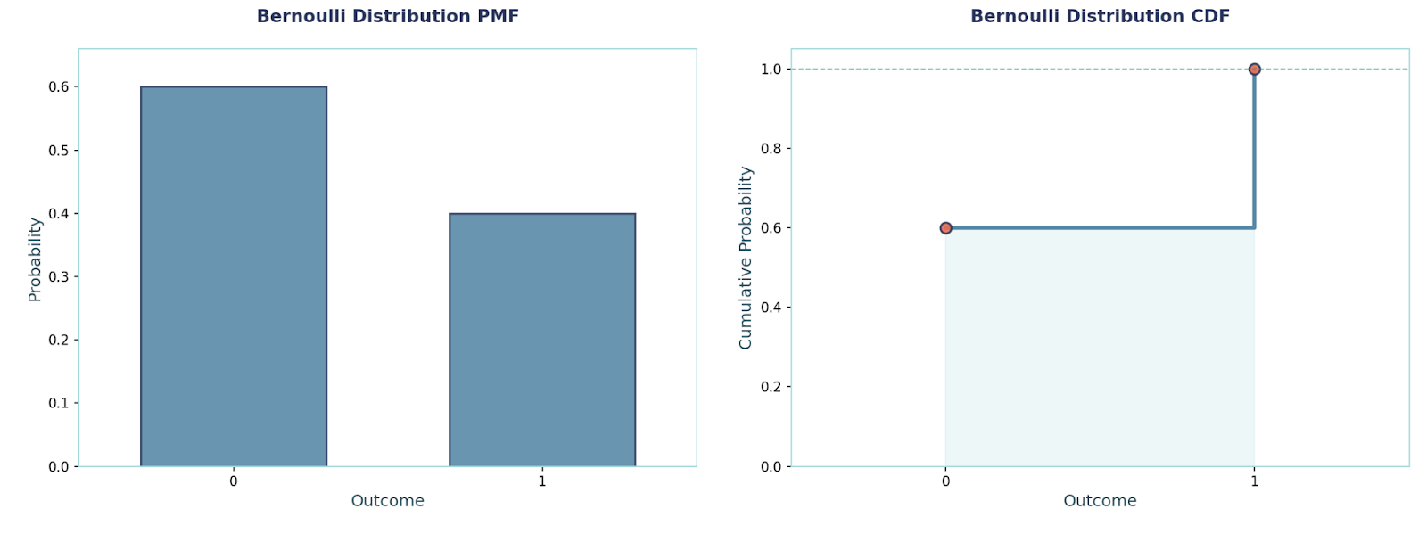

Binomial distribution

This distribution is used when we want to model repeated independent yes/no trials with the same success probability p. We run the trial n times and count how many successes we get. Some examples we use it for are “out of n users, how many converted?”, “out of n parts, how many passed?”, etc. 

The main points I want you to remember for this distribution are the major assumptions: 

1. Each trial has the same probability of success (p)
2. There are a fixed number of trials (n) 
3. The trials are all independent 

PMF:P(X = x) = C(n, x) · pˣ · (1 − p)ⁿ⁻ˣ, x ∈ {0, 1, …, n}, where C is combination

Mean and Variance:E[X] = n·p, Var(X) = n·p·(1 − p)

Example: Let n = 10, p = 0.3.P(X = 4) = C(10, 4) · 0.3⁴ · 0.7⁶ ≈ 0.2001.E[X] = 3, Var(X) = 2.1

The respective code to solve this problem is:

from scipy.stats import binom
n, p, x = 10, 0.3, 4
rv = binom(n, p) # inbuilt binomial distribution method
pmf = rv.pmf(x) # works out P(X=4)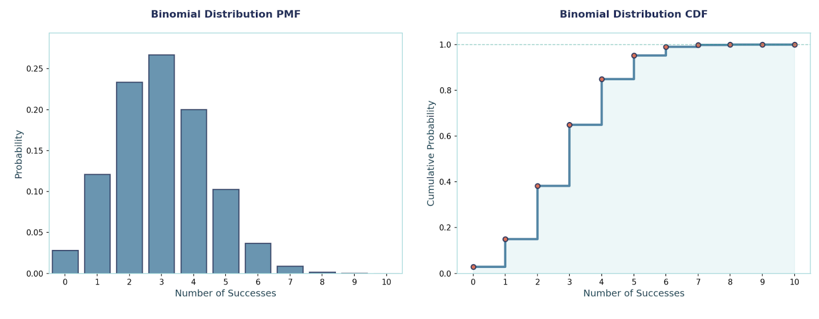

Geometric distribution

This distribution models the number of trials until the first success when each trial succeeds with probability p. We use it for answering questions like “how many attempts until it works?” (first click, first purchase). It is memoryless: past failures don’t change the future.

The memoryless property means the past doesn’t matter, meaning that the probability of future outcomes is the same as if you were starting fresh. Only the geometric and exponential distributions have this property.

PMF:P(X = k) = (1 − p)^(k−1) · p, k ∈ {1, 2, …}

Mean and Variance:E[X] = 1/p, Var(X) = (1 − p)/p²

Example: Let p = 0.2.P(X = 3) = (0.8)² · 0.2 = 0.128.E[X] = 5, Var(X) = 20.

The respective code to solve this problem is:

from scipy.stats import geom
p, k = 0.2, 3
rv = geom(p)  # Inbuilt Geometric distribution method
pmf = rv.pmf(k) # P(X=3)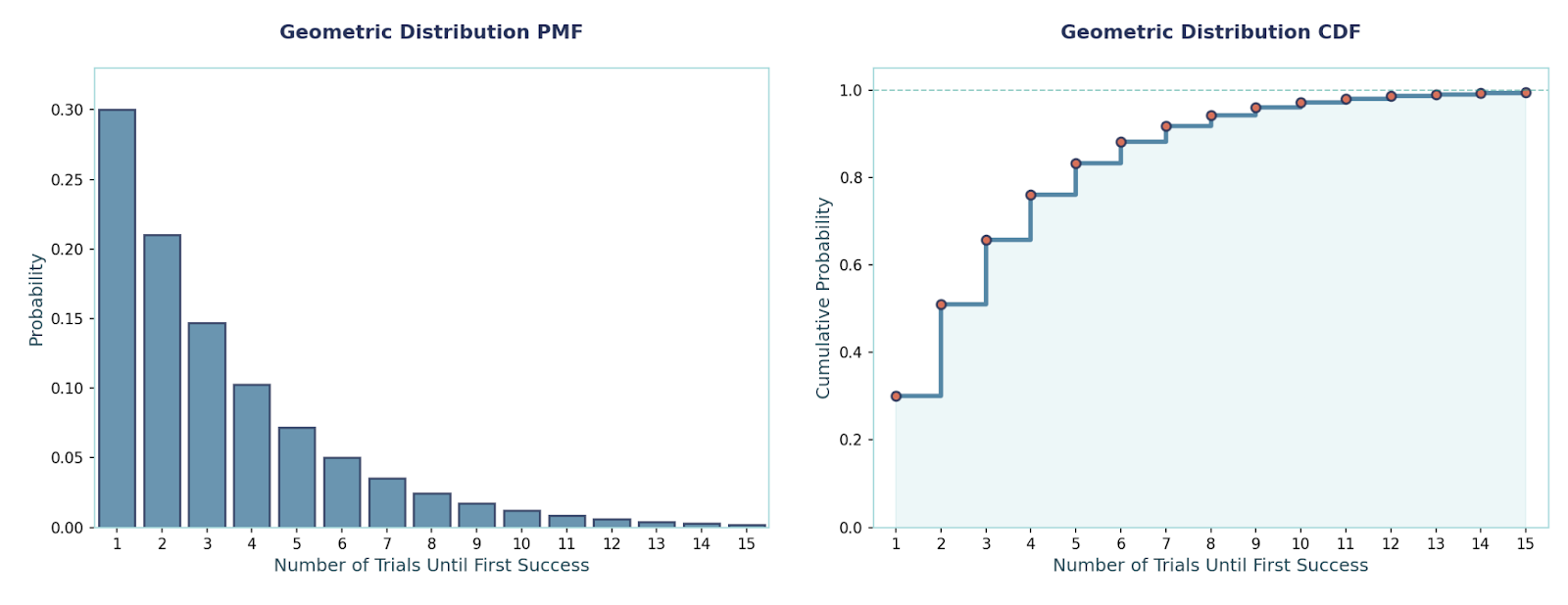

Poisson distribution

Here, the model counts events in a fixed interval when events happen independently at an average fixed rate λ. We use it for scenarios such as for tickets per hour, errors per 1000 requests, or calls per minute — “rare but steady” events. 

An interesting property about this distribution is that it’s mean equals variance.

PMF:P(X = x) = e^(−λ) · λˣ / x!, x ∈ {0, 1, 2, …}

Mean and Variance:E[X] = λ, Var(X) = λ

Example: Let λ = 3, which denotes the average rate of calls a call center gets per hour. P(X = 0) = e^(−3) ≈ 0.0498P(X ≤ 2) = e^(−3) · (1 + 3 + 9/2) ≈ 0.4232

The respective code to solve this problem is:

from scipy.stats import poisson
lam = 3 # average rate
rv = poisson(mu=lam)  # Inbuilt poisson distribution method
P0 = rv.pmf(0) # P(X=0)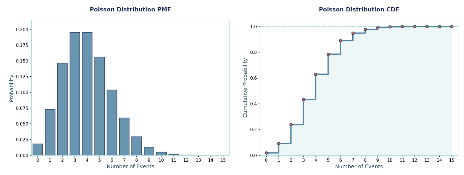

Advanced Distribution Types and Extensions

Now, let’s cover some more advanced discrete probability distributions.

Hypergeometric distribution

This distribution models sampling without replacement from a finite population. From N items with K “successes” (e.g., defectives), we draw n items and count how many successes we get. We use it for things such as quality control on small lots, card draws, or any finite pool where probabilities change after each draw.

PMF:P(X = x) = [C(K, x) · C(N − K, n − x)] / C(N, n), where x ranges from max(0, n − (N − K)) to min(n, K).

Mean and Variance:E[X] = n·(K/N), Var(X) = n·(K/N)·(1 − K/N)·((N − n)/(N − 1))

Example:Let N = 100, K = 8 defectives, n = 10, then probability of at least one defective:P(X ≥ 1) = 1 − C(92, 10)/C(100, 10) ≈ 0.5834

The respective code to solve this problem is:

from scipy.stats import hypergeom
N, K, n = 100, 8, 10
rv = hypergeom(M=N, n=K, N=n)  # Inbuilt hypergeometric distribution method
answer = 1 - rv.pmf(0)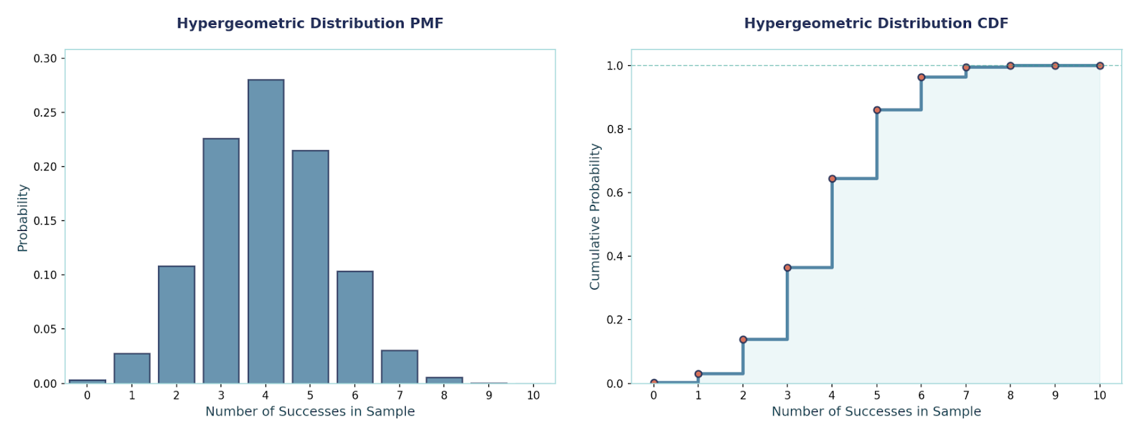

Categorical distribution

This is the multi-class version of a single pick: one trial, exactly one of k classes happens. We use it for multi-class labels (such as {cat, dog, bird}) or any “pick one of k” event. It’s the building block for multi-class classification targets.

PMF:P(X = i) = pᵢ, i ∈ {1, …, k}, Σᵢ₌₁ᵏ pᵢ = 1

Mean and Variance (one-hot view):If you encode the outcome as a one-hot vector Y ∈ {e₁, …, eₖ}, then E[Y] = p, and Cov(Y) = diag(p) − p·pᵀ.

Example:vLet classes = {A, B, C} with p = (0.5, 0.3, 0.2).P(X = B) = 0.3.If stored as one-hot, the mean label vector is [0.5, 0.3, 0.2].

The respective code to solve this problem is:

import numpy as np
from scipy.stats import rv_discrete
classes = np.array(["A", "B", "C"])
p = np.array([0.5, 0.3, 0.2])
rv = rv_discrete(values=(np.arange(len(p)), p)) # Building a categorical random variable over indices {0,1,2}
P_B = rv.pmf(1) # Probability of class "B" (index 1)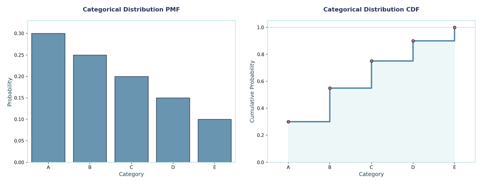

Discrete uniform distribution

This distribution is quite simple; all integers in a range are equally likely. We use it for random integer generators, shuffling, and “no preference” baselines.

PMF:P(X = x) = 1 / (b − a + 1), x ∈ {a, …, b}

Mean and Variance:E[X] = (a + b)/2Var(X) = ((b − a + 1)² − 1)/12

Example:vSuppose we have to pick an integer uniformly from 10 to 15. Therefore, each has probability 1/6Mean = (10 + 15)/2 = 12.5Variance = (6² − 1)/12 = 35/12 ≈ 2.9167

The respective code to solve this problem is:

import numpy as np
from scipy.stats import randint
a, b = 10, 15  # inclusive bounds
rv = randint(low=a, high=b+1)  # note that SciPy randint is [low, high)
xs = np.arange(a, b+1) # PMFs for all outcomes
pmfs = rv.pmf(xs)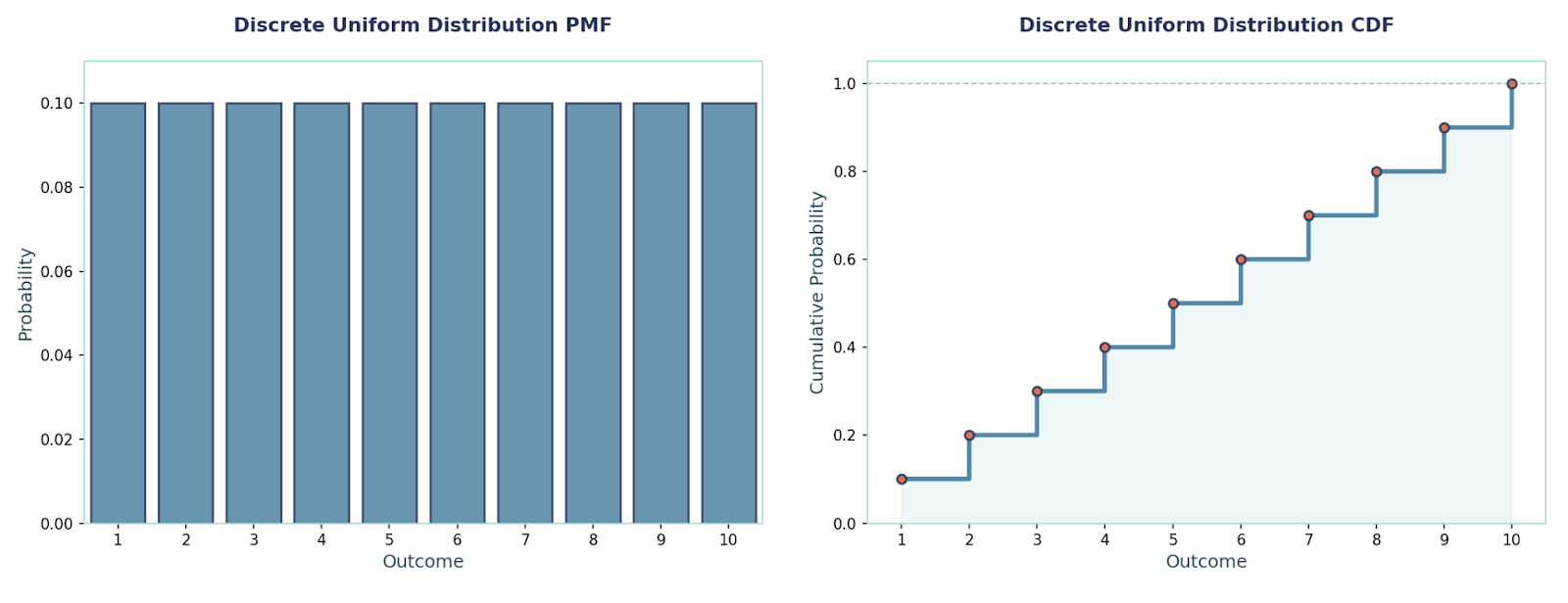

Negative binomial distribution

This models the number of trials needed to achieve r successes when each trial is independent and has the same success probability p. Honestly, it is a natural generalization of the geometric distribution (which is the special case r = 1). We use it when we care about when the r-th success happens. Some example scenarios are “On which customer will we record our 3rd purchase?”, “How many calls until we close 5 deals?”, etc.

PMF:P(X = k) = C(k−1, r−1) · pʳ · (1 − p)^(k−r), k = r, r+1, r+2, …

Mean and Variance:E[X] = r/pVar(X) = r·(1 − p)/p²

Example: Suppose each trial succeeds with probability p = 0.3, and we want the 3rd success (r = 3).

Probability the 3rd success occurs on trial k = 7:P(X = 7) = C(6, 2) · (0.3)³ · (0.7)⁴ = 15 × 0.027 × 0.2401 ≈ 0.09724.

The respective code to solve this problem is:

from scipy.stats import nbinom
p, r, k = 0.3, 3, 7
rv_failures = nbinom(r, p)  # Inbuilt method for negative binomial distribution
P_X_eq_k = rv_failures.pmf(k - r)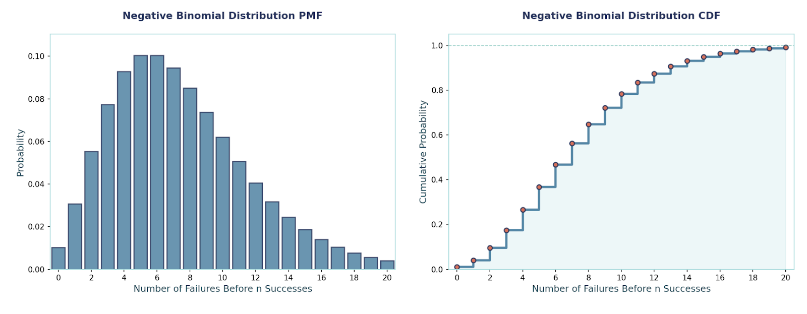

Final Thoughts

All in all, Discrete probability distributions are the backbone of modeling countable outcomes, helping us quantify uncertainty in everything from quality control to machine learning. 

We have learned a lot about discrete probability distributions. To progress further, I would highly recommend reading our tutorial on Probability Distributions in Python, as well as starting to move towards continuous distributions such as Gaussian and Exponential Distribution.