Joint Probability: Theory, Examples, and Data Science Applications

When a weather analyst predicts a severe storm, they're not just forecasting heavy rain or strong winds independently – they're assessing the probability that both weather conditions will occur together. This scenario illustrates joint probability – the likelihood of two events happening simultaneously. 

In this article, we'll explore how joint probability works, examine formulas for both dependent and independent events, work through practical examples, and see how this concept is applied in data science and machine learning. For a handy reference to basic probability definitions and rules, check out DataCamp's Introduction to Probability Rules Cheat Sheet. 

What is Joint Probability?

Joint probability represents the likelihood of two (or more) events occurring at the same time. Mathematically, we denote this as P(A∩B), which is read as "the probability of A intersection B" or simply "the probability of A and B."

To understand joint probability, we first need to establish some context:

• Sample space: The set of all possible outcomes in an experiment.
• Event: A subset of outcomes from the sample space.
• Marginal probability: The probability of a single event occurring, regardless of other events.
• Conditional probability: The probability of an event occurring given that another event has already occurred.

Joint probability differs significantly between independent and dependent events:

• Independent events: Events where the occurrence of one has no effect on the probability of the other. For example, flipping two coins—the outcome of the first flip doesn't influence the second.
• Dependent events: Events where the occurrence of one affects the probability of the other. For example, drawing cards without replacement—removing one card changes the composition of the remaining deck.

We can visualize joint probability using a Venn diagram, where the overlapping region represents the intersection of events—the scenarios where both events occur simultaneously:

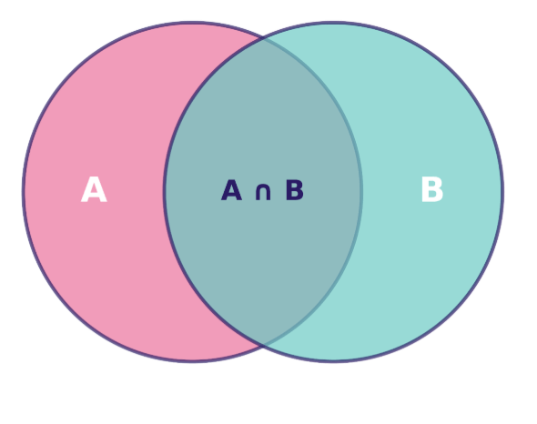
Venn diagram showing the relationship between sets A and B, with their intersection A ∩ B highlighted. Image by Author.

This overlapping region's area, relative to the total sample space, gives us P(A∩B)—the joint probability we're seeking to calculate.

The Joint Probability Formula and Key Properties

Understanding how to calculate joint probability requires different approaches depending on whether events are independent or dependent. Let's examine both scenarios and explore the rules that govern these calculations.

Joint probability for independent events

When two events are independent, calculating their joint probability becomes straightforward. Since neither event influences the other, we can simply multiply their individual probabilities:

P(A∩B) = P(A) × P(B)

This multiplication rule applies because independence means that knowing one event occurred provides no information about the likelihood of the other event.

Example: Consider flipping two fair coins. The probability of getting heads on the first coin is 1/2, and the probability of getting heads on the second coin is also 1/2. Since these events are independent (the first flip doesn't affect the second), the probability of getting heads on both coins is:

This means there's a 25% chance of flipping two heads in succession.

Joint probability for dependent events

When events are dependent, we must account for how the first event affects the probability of the second. This requires using conditional probability in our calculation:

Here, P(B|A) represents the probability of event B occurring given that event A has already occurred.

Example: Imagine drawing two cards from a standard deck without replacement. What's the probability of drawing two aces?

• The probability of drawing an ace on the first draw is P(Ace₁) = 4/52 = 1/13
• After drawing an ace, only 3 aces remain in a deck of 51 cards, so P(Ace₂|Ace₁) = 3/51 = 1/17
• Therefore:

This illustrates how dependence significantly affects the joint probability calculation.

Multiplication rule and chain rule

The calculations above demonstrate the multiplication rule of probability. This rule extends to more than two events, allowing us to calculate joint probabilities for multiple events using a chain of conditional probabilities:

This is known as the chain rule, which provides a systematic way to break down complex joint probabilities into manageable pieces.

Example: Consider the probability of drawing three hearts in succession from a standard deck without replacement:

• P(Heart₁) = 13/52 = 1/4
• P(Heart₂|Heart₁) = 12/51
• P(Heart₃|Heart₁ ∩ Heart₂) = 11/50
• P(Heart₁ ∩ Heart₂ ∩ Heart₃) = 1/4 × 12/51 × 11/50 = 11/850

The chain rule becomes particularly valuable in data science when modeling sequences of events or working with multi-stage processes.

Examples to Illustrate Joint Probability

To solidify our understanding of joint probability, let's work through some classic examples and explore practical applications that demonstrate how these concepts operate in various contexts.

Classical examples

Dice rolls

Imagine rolling two six-sided dice. What's the probability of rolling a 4 on the first die and a 6 on the second die?

Since the outcome of the first die doesn't affect the second die, these are independent events:

• P(First die = 4) = 1/6
• P(Second die = 6) = 1/6
• P(First die = 4 ∩ Second die = 6) = 1/6 × 1/6 = 1/36

This tells us there's approximately a 2.78% chance of this specific combination occurring.

Card drawing

Let's calculate the probability of drawing a red card followed by an Ace from a standard 52-card deck without replacement.

Since we're drawing without replacement, these events are dependent:

• P(Red card on first draw) = 26/52 = 1/2
• P(Ace on second draw | Red card on first draw) = 3/51 if the first card was a red Ace, or 4/51 if the first card was not an Ace

To handle this properly, we need to consider both scenarios:

• P(Red non-Ace then Ace) = P(Red non-Ace) × P(Ace | Red non-Ace) = 24/52 × 4/51 = 24/663
• P(Red Ace then another Ace) = P(Red Ace) × P(Ace | Red Ace) = 2/52 × 3/51 = 1/442

Therefore, the total joint probability is: P(Red card ∩ Ace on second draw) = 24/663 + 1/442 = (24×2 + 3)/1326 = 51/1326 = 1/26

The probability is approximately 3.85%.

Marbles in a bag

Consider a bag containing 5 blue marbles and 3 green marbles. Let's calculate the probability of drawing two blue marbles under two different scenarios.

With replacement:

• P(Blue on first draw) = 5/8
• P(Blue on second draw) = 5/8 (unchanged because the first marble is replaced)
• P(Blue ∩ Blue) = 5/8 × 5/8 = 25/64 ≈ 39.06%

Without replacement:

• P(Blue on first draw) = 5/8
• P(Blue on second draw | Blue on first draw) = 4/7
• P(Blue ∩ Blue) = 5/8 × 4/7 = 20/56 = 5/14 ≈ 35.71%

This comparison highlights how the dependency created by not replacing the marbles reduces the joint probability.

Real-world applications

Medical diagnosis

Joint probability is vital in medical contexts when assessing multiple symptoms or test results. Consider a diagnostic scenario where physicians need to assess patients with symptoms A and B for a specific condition.

Based on historical data:

• P(Symptom A) = 0.30 (30% of the population shows symptom A)
• P(Symptom B) = 0.25 (25% of the population shows symptom B)
• P(Symptom A ∩ Symptom B) = 0.12 (12% show both symptoms)

This joint probability helps physicians assess the likelihood of different conditions. It's worth noting that P(A ∩ B) is not equal to P(A) × P(B) = 0.30 × 0.25 = 0.075, which indicates these symptoms are not independent—knowing a patient has one symptom increases the likelihood they have the other.

Financial risk modeling

Investment analysts often need to evaluate the joint probability of multiple market conditions occurring together. Consider an analyst assessing the risk of both a stock market decline and rising interest rates within the next quarter.

If their models suggest:

• P(Stock market decline) = 0.35
• P(Rising interest rates) = 0.60
• P(Stock market decline | Rising interest rates) = 0.45

The joint probability calculation would be: P(Stock market decline ∩ Rising interest rates) = 0.60 × 0.45 = 0.27

This 27% probability helps quantify portfolio risk and guides hedging strategies to protect against this scenario.

These examples demonstrate how joint probability serves as a powerful tool for quantifying uncertainty in diverse fields, whether analyzing simple games of chance or making complex decisions in medicine and finance.

Joint Probability and Conditional Probability

Joint and conditional probabilities are closely intertwined concepts that allow us to analyze complex scenarios involving multiple events. Understanding their relationship provides powerful tools for probabilistic reasoning.

The fundamental relationship

The relationship between joint and conditional probability is expressed by the formula:

Rearranging this equation, we can express joint probability in terms of conditional probability:

This relationship shows that we can calculate joint probability if we know the marginal probability of one event and the conditional probability of the other given the first.

Similarly, we could also write:

Both formulations are valid and equivalent, demonstrating the symmetrical nature of joint probability.

Relevance to Bayes' Theorem

The relationship between joint and conditional probability is central to Bayes' Theorem, a fundamental tool in probabilistic inference:

Bayes' Theorem allows us to "reverse" conditional probabilities—if we know P(B|A), we can calculate P(A|B). This proves invaluable when we have information about one conditional relationship but need to reason about the reverse relationship.

For example, medical tests often provide information about P(Positive Test|Disease), but doctors need to determine P(Disease|Positive Test). Bayes' Theorem bridges this gap by incorporating joint probability:

Applications in Data Science

Joint probability forms the foundation for numerous data science techniques and applications. Understanding how multiple events interact helps data scientists build more accurate models and make better predictions in various domains.

Predictive modeling

Joint probability is fundamental to many classification algorithms, particularly Naive Bayes classifiers. These popular machine learning models calculate the probability of different outcomes based on the presence of multiple features.

The Naive Bayes approach applies Bayes' Theorem with a "naive" assumption that features are conditionally independent. This simplifies joint probability calculations:

Despite this simplifying assumption, Naive Bayes classifiers work remarkably well for:

• Text classification and spam filtering
• Sentiment analysis
• Medical diagnosis
• Customer segmentation

This approach is computationally efficient and often performs surprisingly well even when the independence assumption doesn't strictly hold.

Risk assessment

Joint probability plays a crucial role in fraud detection systems, where multiple risk factors must be evaluated together. Modern fraud detection algorithms analyze combinations of suspicious behaviors to identify potentially fraudulent transactions.

Consider an online payment system that monitors various signals:

• Transaction amount
• Geographic location
• Time of transaction
• Device information
• User behavior patterns

While each signal alone might not indicate fraud, specific combinations (their joint occurrence) can significantly increase suspicion. For instance, a large transaction, from a new device, in a foreign country, at an unusual time represents a joint event with potentially high fraud probability.

This joint probability assessment enables more sophisticated risk scoring than evaluating each factor in isolation, reducing both false positives and false negatives.

Machine learning

Joint probability concepts are central to many advanced machine learning models, including:

Bayesian Networks: These graphical models represent variables and their probabilistic relationships. They enable reasoning about complex joint probability distributions by breaking them down into simpler conditional probabilities. Bayesian networks are widely used in:

• Medical diagnosis systems
• Genetic analysis
• Decision support systems
• Causality modeling

Hidden Markov Models (HMMs): These sequential models use joint probabilities to model systems where the underlying state is hidden but produces observable outputs. Applications include:

• Speech recognition
• Natural language processing
• Biological sequence analysis
• Financial time series modeling

Probabilistic Graphical Models: These encompass a broader class of models that use graph structures to encode complex joint probability distributions. They're essential tools for:

• Image recognition
• Recommendation systems
• Anomaly detection
• Reinforcement learning

Through these applications, joint probability enables data scientists to build models that capture the complex interdependencies in real-world data, leading to more accurate predictions and better decision-making under uncertainty.

How People Can Misinterpret Joint Probability

Despite its usefulness, joint probability is often misunderstood or misapplied. Let's examine some common misconceptions and how to avoid them.

Confusing joint probability with conditional probability

One of the most frequent mistakes is confusing P(A∩B) with P(A|B). While they're related, they represent different concepts:

• Joint probability P(A∩B) answers: "What's the probability that both A and B occur?"
• Conditional probability P(A|B) answers: "Given that B has occurred, what's the probability that A occurs?"

For example, the probability that a person both has diabetes and is over 65 (joint) is different from the probability that a person has diabetes given that they're over 65 (conditional).

This distinction matters in many analytical contexts. For instance, when a data scientist reports that "5% of users both clicked on an ad and made a purchase," this joint probability is very different from "40% of users who clicked on an ad made a purchase," which is a conditional probability.

Incorrectly assuming independence

Another common error is automatically assuming that P(A∩B) = P(A) × P(B) without verifying that events are truly independent. This assumption can lead to significant errors when events are actually dependent.

For example, in market analysis, assuming independence between purchasing product A and product B might lead to incorrect inventory planning if these products are complementary (like printers and ink) or substitutes (like different brands of the same item).

Testing for independence is crucial—if P(A∩B) ≠ P(A) × P(B), the events are dependent, and more careful joint probability calculations are required.

Ignoring marginal probabilities

When working with joint probabilities, analysts sometimes focus exclusively on the intersection while ignoring the overall frequency of individual events. This can lead to misleading conclusions about the strength of relationships.

For instance, discovering that 90% of customers who bought products A and B also bought product C might seem impressive. However, if 89% of all customers buy product C regardless, the apparent relationship is much weaker than it initially appeared.

Always compare joint probabilities against relevant marginal probabilities to avoid overstating relationships between events. The lift ratio—the ratio of the joint probability to the product of marginal probabilities—offers a more accurate measure of association:

A lift value greater than 1 indicates events occur together more often than would be expected if they were independent.

Understanding these common pitfalls helps data scientists apply joint probability correctly and derive meaningful insights from probabilistic analysis.

Advanced Topics and Further Considerations

As data scientists progress in their careers, they'll encounter more sophisticated applications of joint probability. Let's explore some advanced concepts that build upon the foundations we've established.

Joint probability in high-dimensional spaces

When dealing with modern machine learning problems, data scientists often work with dozens or even hundreds of variables simultaneously. In these high-dimensional spaces, calculating and representing joint probabilities becomes challenging.

The number of parameters needed to specify a joint distribution grows exponentially with the number of variables—a phenomenon known as the "curse of dimensionality." For example, a joint distribution of 10 binary variables requires 2¹⁰ - 1 = 1,023 parameters to specify completely.

To manage this complexity, data scientists employ techniques like:

• Dimensionality reduction
• Variable selection
• Conditional independence assumptions
• Factorized representations (like Bayesian networks)

These approaches make high-dimensional joint probability calculations tractable for practical applications in areas like computer vision, genomics, and natural language processing.

Joint probability distributions

Our examples so far have mostly involved discrete events, but joint probability extends naturally to continuous variables through joint probability distributions.

For discrete variables, we work with joint probability mass functions (PMFs), which specify the probability that each combination of random variables takes on specific values:

For continuous variables, we use joint probability density functions (PDFs). Unlike PMFs, PDFs don't directly give probabilities but must be integrated over regions to find the probability that the variables fall within those regions:

Common joint distributions include:

• Multivariate normal distribution
• Multivariate t-distribution
• Dirichlet distribution
• Multinomial distribution

Understanding these distributions enables more sophisticated modeling of relationships between continuous variables in fields like economics, bioinformatics, and environmental science.

Practical tools for computing joint probability

Several software tools and programming languages offer functions and libraries for working with joint probabilities:

Python:

• NumPy and SciPy provide functions for multivariate probability distributions

• Pandas offers powerful tools for empirical joint probability calculations

• Libraries like PyMC3 and PyStan implement Bayesian modeling with joint distributions

R:

• Base R includes many multivariate distribution functions

• Packages like copula enable modeling complex dependence structures

• bnlearn supports Bayesian network analysis

SQL:

• GROUP BY clauses with COUNT functions can calculate empirical joint probabilities

• Window functions enable more complex probabilistic analysis

• Modern databases support statistical functions for probability calculations

These tools make it practical to apply joint probability concepts to large datasets, enabling data scientists to build sophisticated probabilistic models for complex problems.

To deepen your understanding of joint probability and its applications in Bayesian analysis, DataCamp offers several excellent courses:

• Fundamentals of Bayesian Data Analysis in R - Learn how to apply Bayesian methods to common data analysis problems
• Bayesian Modeling with RJAGS - Master practical Bayesian modeling techniques using the JAGS framework in R
• Bayesian Data Analysis in Python - Develop skills for implementing Bayesian approaches to data analysis using Python

These courses will help you build on the concepts covered in this article and apply joint probability techniques to solve real-world data science problems.

Conclusion

As we've seen throughout this article, joint probability is a fundamental statistical concept with wide-ranging applications across numerous data science fields. DataCamp's resources, like those shared in the 40+ Python Statistics for Data Science Resources, provide excellent pathways to strengthen your understanding. This comprehensive collection includes specific recommendations for learning probability theory, Bayesian thinking, and other statistical concepts that build upon joint probability.

For those preparing for data science roles, our Top 35 Statistics Interview Questions and Answers guide offers valuable practice with joint probability questions alongside other important statistical concepts.  I also think that our Probability Puzzles in R course is a fun option.