MODE() Function in Excel: Find the Most Frequent Number

Whether you're summarizing survey responses, tracking popular product quantities, or analyzing repeated entries in any dataset, The MODE() function in Excel tells you which number appears most frequently—something that’s often more relevant than an average or a median when you're looking for patterns.

In this guide, we’ll show you how to use the MODE() function effectively, including how it differs from Excel’s other mode-related functions. You’ll learn how to apply it in real scenarios, avoid common pitfalls, and expand your skills with related tools. Let’s start with the basics.

What Is the MODE() Function in Excel?

Before diving into practical use, let’s start with the basics: the MODE() function in Excel is your go-to tool for finding the most frequently occurring number in a range of values. Whenever you’re faced with a list and want to quickly figure out which number pops up the most, MODE() offers a simple solution.

This function becomes especially valuable when you need to summarize data, spot trends, or check for repeated entries. Whether you’re analyzing survey responses, reviewing inventory numbers, or dealing with any scenario where the most common value matters, MODE() makes the process straightforward.

Here’s the basic syntax:

=MODE(number1, [number2], ...)

Here, number1, [number2], … represent numbers or ranges where you want to check for the mode.

It’s important to note that MODE() only works with numbers. If your data includes text or empty cells, Excel will simply skip over those entries.

Understanding How MODE() Works in Excel

Now that you know what MODE() is, let’s see how it actually operates. In this section, you’ll learn how MODE() processes your data and what to expect from its results.

MODE() examines your list, counts how often each number appears, and returns the one with the highest frequency. If two or more numbers are tied for being most frequent, Excel returns the first one it finds in your data range.

How to Use MODE() with Real Data in Excel

Now that you understand how MODE() works and how it compares to its counterparts, let’s put it into practice with real-world examples. In this section, you’ll see how to apply MODE() to find the most common values in various scenarios.

Example 1: Finding the most common test score

Suppose you have student test scores in cells A2 to A11:

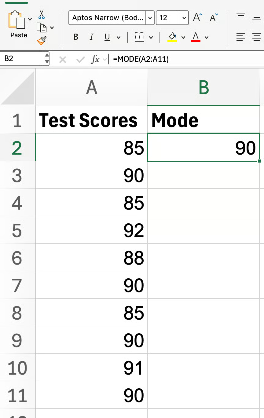
To find the most common score, enter:

=MODE(B2:B11)

You’ll get 85 or 90 depending on which appears first, since both values occur several times. Remember, MODE() only returns the first mode it detects. If you want to see every mode in cases of a tie, that’s when MODE.MULT() comes in handy.

Example 2: Using MODE() with non-contiguous ranges

What if your data isn’t in a single continuous block? No problem! MODE() allows you to use multiple arguments. For example:

=MODE(A1:A5, C1:C5)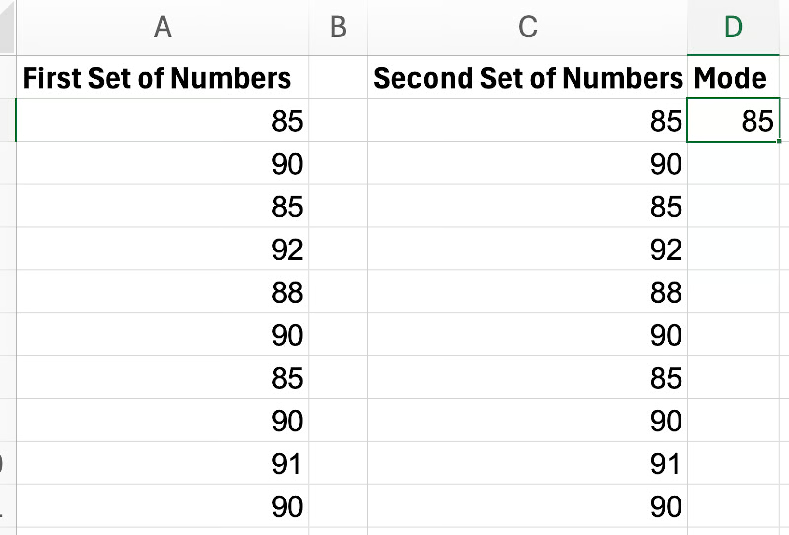

Excel will then search across both ranges for the most frequent number.

Example 3: What happens with no repeat values?

You might be curious what MODE() does when there’s no repeated value. If every value in your range is unique, MODE() returns an #N/A error.

Suppose A1:A5 contains 10, 20, 30, 40:

=MODE(A2:A5)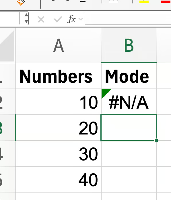

Since no number repeats, you’ll see #N/A as the result.

With these examples, you can see how MODE() adapts to different data layouts and situations. I know there is still some nuance in all this, so I’ll put some of these and other common scenarios into a table:

Common Issues and Tips in Excel

You might encounter a few common scenarios. In this section, we’ll look at how to handle errors, deal with non-numeric data, and work efficiently with large datasets.

Handling errors

If you get a #N/A error, as we did above, it means there’s no mode in your data. To make your formulas more user-friendly, you can wrap MODE() with IFERROR():

=IFERROR(MODE(A1:A10), "No mode")

This way, you’ll see “No mode” instead of an error, which can be a little unsightly.

Dealing with non-numeric data

MODE() only considers numbers. It ignores text, blank cells, and logical values. If your range mixes numbers and text (like “N/A” entries in survey data), MODE() will simply skip the non-numeric items.

Using MODE() for large datasets

MODE() works well even with large ranges of numbers. Just keep in mind: if your data contains multiple modes, MODE() will only return the first one it finds. For a complete list of all modes, especially in bigger datasets, switch to MODE.MULT().

By handling these scenarios, you’ll ensure your MODE() results are accurate and your formulas robust. Now, let’s see how MODE() looks in a real spreadsheet.

MODE() vs. MODE.SNGL() and MODE.MULT()

With the basics under your belt, you might be wondering: what’s the difference between MODE(), MODE.SNGL(), and MODE.MULT()? In this section, we’ll compare these related functions so you can choose the right one for your needs.

• MODE(): This is the original function, kept for compatibility. In newer Excel versions, you’ll often see MODE.SNGL() instead, but both serve the same purpose—they return a single mode value.

• MODE.SNGL(): Works just like MODE(), giving you the first mode it finds in your data.

• MODE.MULT(): Takes things a step further by returning an array of all modes when there’s a tie. To use it, you’ll need to enter it as an array formula (using Ctrl+Shift+Enter in legacy Excel).

Most of the time, MODE() or MODE.SNGL() is all you need for quick answers. But if your dataset could have multiple equally frequent values and you want to see them all, MODE.MULT() is the function to use.

Related Statistical Functions in Excel

As you continue building your Excel toolkit, you’ll notice that MODE() often appears alongside other summary statistics functions. Let’s highlight a few that pair well with MODE():

• MEDIAN() – returns the middle value in a dataset

• AVERAGE() – calculates the arithmetic mean

• COUNTIF() – counts how many times a specific value appears, useful for checking frequencies manually

And if you’re working with data that might have more than one mode, don’t forget about MODE.MULT(). 

Conclusion

As we’ve seen, MODE() is a useful yet simple tool for finding the most common number in any list. Whether you’re summarizing survey results, tracking sales, or analyzing repeated entries, MODE() delivers fast insights with just a single formula. 

To take your Excel skills further, explore other statistical functions like MEDIAN(), AVERAGE(), and COUNTIF(). Combining these tools will help you summarize, analyze, and truly understand your data from every angle. And remember to enroll in our As a next step, take our Data Analysis in Excel course to keep refining your skills.