Excel MATCH() Function: How to Find the Position of a Value in a Range

In this article, I will show what makes Excel's MATCH() function unique compared to Excel’s other lookup functions.

What makes MATCH() unique is that, unlike VLOOKUP() or HLOOKUP(), which return actual values, MATCH() gives us the position of a value, which can be extremely useful in many situations - let’s see how.

The Quick Answer

To find the position of a value using the MATCH() function:

• Click on an empty cell where you want the result

• Type =MATCH(

• Then write the lookup value in inverted commas

• Select the lookup_array.

• Enter the match type (0 for exact match) and hit Enter.

For example, I have a list of fruits and their sales in the A2:B6 range, and I want to find the position of Orange in this list. To do so, I write the following formula and press Enter: 

=MATCH(“Orange”, A2:A6, 0)

This will display 4 because Orange is the fourth fruit in the list.

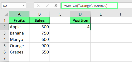
Use the MATCH() function. Image by Author.

Understanding Excel MATCH()

There’s more than one way to use MATCH() and how we use it can change what we get from it. Let’s understand this in more detail so you can decide what works best for you.

What is the MATCH() function?

The MATCH() function in Excel returns the position of a value in a list. Instead of giving the actual value, it tells us where that value is located. This works best when we have to know the position rather than the value itself, especially for dynamic lookups.

Syntax of the MATCH() function

The syntax of MATCH() is:

MATCH(lookup_value, lookup_array, [match_type])

Here: 

• lookup_value is the value we’re looking for in lookup_array.

• lookup_array is the list that searches for that value.

• match_type (optional) tells how to search. 1 (default) returns the largest value less than or equal to the lookup_value (the list must be sorted in ascending order). 0 returns an exact match. And -1 returns the smallest value greater than or equal to what you’re looking for (the list must be sorted in descending order).

Key things to know about the MATCH() function 

Before you use the MATCH() function, a few small things are worth knowing. They’ll help you avoid mistakes and make things a bit easier:

• MATCH() doesn’t care about uppercase or lowercase letters, so apple, Apple, and APPLE are treated the same. 

• If we work with text and set the match_type to 0, we can use wildcards such as an * to represent multiple characters and a ? to represent a single character. 

• If MATCH() cannot find our desired value, it will return an #N/A error.

Basic Examples of Using Excel MATCH()

Now that we know what the MATCH() function is and how it works, let's see how we can use it with a few examples: 

Example 1: Finding the position of a number

Let's say I have a range of numbers in cell A2:A7 and want to find the position of the number 40 within a list. For this, I can use the MATCH() function like this:

=MATCH(40, A2:A7, 0)

Or I can also use a cell reference for the lookup value.

=MATCH(D1, A2:A7, 0)

Looking at the left Excel heading, you'll see that the number 40 is in row 6. But the result shows 5. That’s because we start counting from A2. So, when Excel counts from there, it gives us 5 instead of 6.

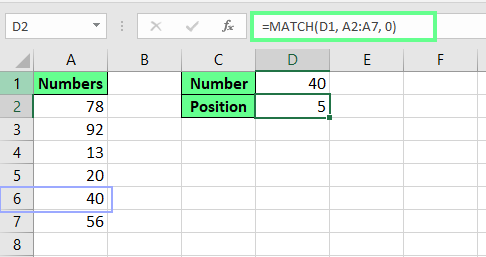
Find the position of a number using the MATCH() function. Image by Author.

Example 2: Finding the position of a text value

I have a list of Players in cell A2:A7 and their Scores in cell B2:B7 sorted in ascending order, and I want to find the position of the player Emily. For this, my formula looks like this:

=MATCH(E1,A2:A6, 0)

This formula searches for the value in cell D1 in the range A2:A7 and returns 3 because Emily is the third player in the list.

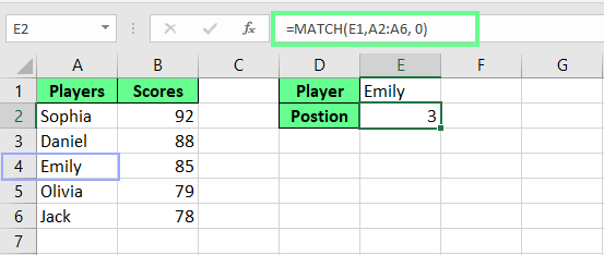
Find the position of a text using the MATCH() function. Image by Author.

Fuzzy Matching and Wildcard Matching in Excel

Sometimes, the data we work with isn’t perfect — there may be typos, different spellings, or messy formats. In such cases, fuzzy and wildcard matching can help tidy things up.

Fuzzy match 

Fuzzy matching finds records from different lists that are similar but not exactly the same. This is useful when there is a slight variation or typos like Frank vs. Feank.

I have two datasets: Customer Order list and Loyalty Program Members. And I want to check which customers’ Orders are already in the Loyalty Program, even if there are some variations due to typos, nicknames, or formatting differences. A VLOOKUP() won’t work here because the names don’t match exactly.

Step 1: Convert data into tables

• Select Customer Orders, press Ctrl + T.  

• Select Loyalty Program Members, press Ctrl + T.

Make sure there is space between the two tables to keep them separate.

Step 2: Load data into Power Query  

• Click anywhere inside Customer Orders, and name it Orders_Table.  
• Go to Data > Get Data > From Table/Range.  
• Click Close & Load to load it into Power Query.  
• Repeat Steps 1-3 for Loyalty Program Members, and name it Loyalty_Table but this time select Close & Load To and load it into the same Excel sheet.

Now, both tables are loaded into Power Query.

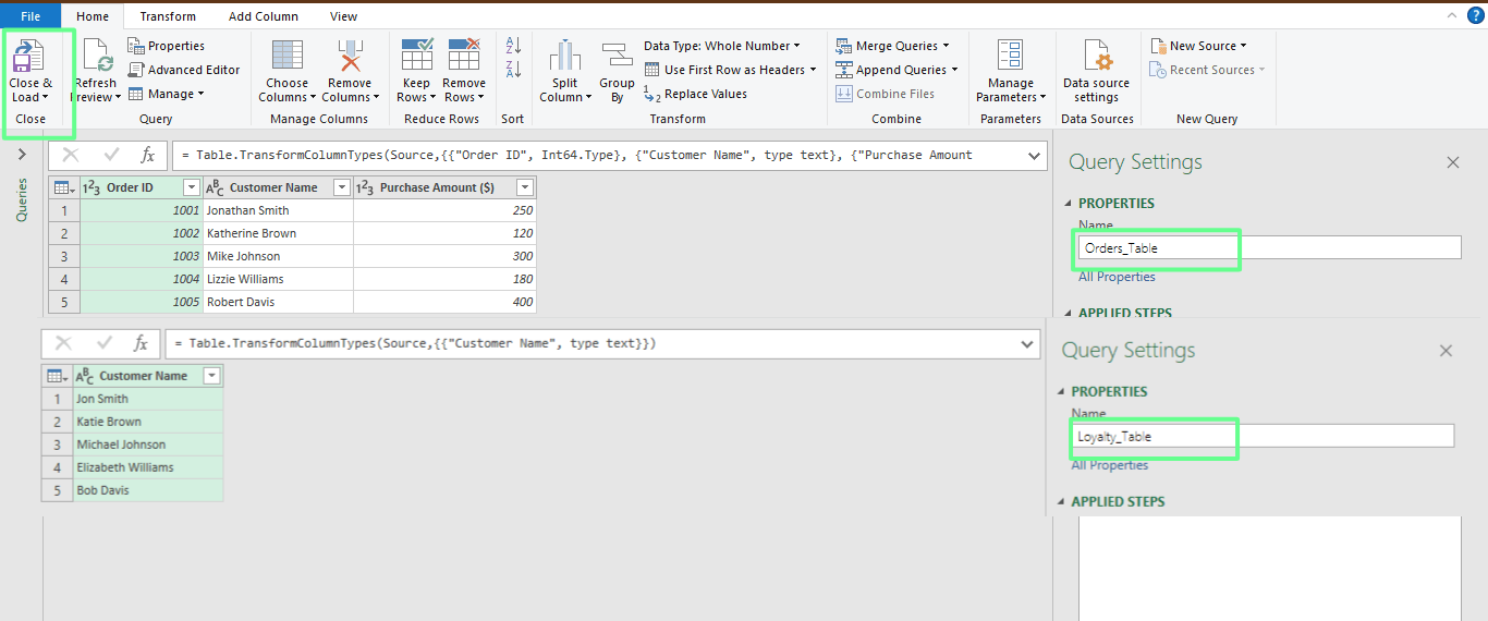
Load the tables in Power Query. Image by Author.

Step 3: Merge tables using fuzzy matching  

• Go to Data > Get Data > Combine Queries > Merge Queries.  
• In the Merge window, select the first table (Orders_Table) and the second table (Loyalty_Table)   
• Select the Customer Name column in both tables.  
• Check the Use Fuzzy Matching box.  
• Click the dropdown and set the similarity threshold to 0.3 (Allows some variations like typos or nicknames).

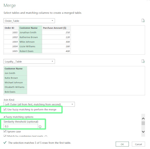
Use fuzzy match to merge the tables. Image by Author.

Power Query will now match names that are similar rather than exact.  

Step 4: Expand the matched data

• Click the expand icon next to the matched column.
• Select Customer Name from Loyalty_Table and click OK.  
• Close & Load the results back into Excel.  

You can see in the image below that fuzzy lookup has automatically matched customers with name variations.

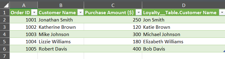
Tables merged using the fuzzy match. Image by Author.

Wildcard match

Wildcard matching helps us find names or values when we only know part of what we're looking for. It helps when we work with similar entries or fuzzy memories. There are two wildcards we can use:

• * matches any number of characters (E.g., Jo* matches John and Jonathan).

• ? matches just one character (E.g., J?ck matches Jack but not Jake).

Here’s how they work:

• A* matches anything that starts with A.

• *A matches anything that ends with A.

• *A* matches anything that contains A anywhere in the cell.

For example, to find the name of the person whose name ends with e, I use:

=MATCH("*e", A2:A11, 0)

You can see in the image below that the formula returns 3 because the name Charlie ends with e.

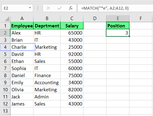
Find the position using wildcards. Image by Author.

Combining MATCH() with Other Excel Functions

MATCH() gets even more helpful when we pair it with other functions. It makes our formulas more flexible and easier to update. Let’s see how.

Combining MATCH() with INDEX()

MATCH() is often paired with INDEX() for powerful lookups. Unlike VLOOKUP(), which can only search from left to right, INDEX() and MATCH() work together to look up values in any direction.

For example, I have a list of players and their scores, and I want to find Brian’s score. For this, I use the following formula:

=INDEX(B2:B11,MATCH("Brian",A2:A11,0))

And with cell reference, it looks like:

=INDEX(B2:B11, MATCH(E1, A2:A11, 0))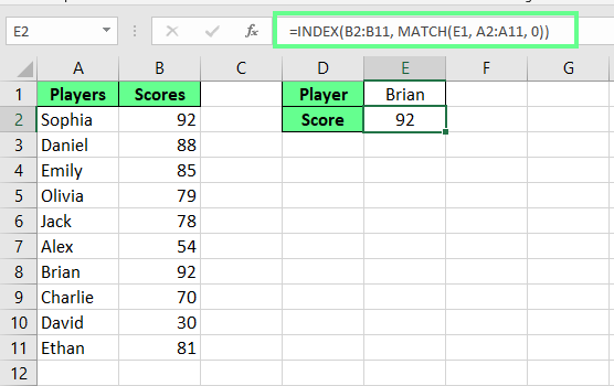

Combine INDEX() and MATCH(). Image by Author.

Using MATCH() for dynamic column selection in VLOOKUP()

We know VLOOKUP() requires manually entering the column number where the result is. If the columns change, we have to update the formula. To avoid this, we can use MATCH() to find the right column automatically.

For example, I have a dataset and I want to find out the team name of Emily. With VLOOKUP(), the formula looks like this:

=VLOOKUP(F1, A2:C12, 3, FALSE)

This formula can only search from left to right, and the column number 3 is fixed, so if columns change, I have to update the formula manually.

So instead of hardcoding the column number in VLOOKUP(), we can combine MATCH() like this:

=VLOOKUP(F1, A2:C12, MATCH("Team", A1:C1, 0), FALSE)

In this formula, MATCH("Team", A1:C1, 0) finds which column contains Team and returns it. Then, VLOOKUP(F1, A2:C4, 3, FALSE) pulls the data from the third column instead of a fixed number.

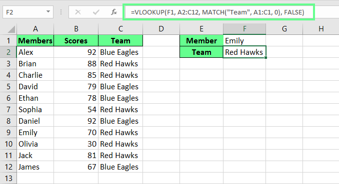
Combine VLOOKUP() and MATCH(). Image by Author.

Case-sensitive MATCH() using EXACT()

By default, MATCH() ignores uppercase and lowercase letters, so Apple and apple will be treated as the same. If we need a case-sensitive search, we have to combine MATCH() with the EXACT() function like this: 

=MATCH(TRUE, EXACT(A2:A7, D2), 0)

This is an array formula, so press Ctrl + Shift + Enter. In this formula, EXACT(A2:A4, "Emily") checks each name and returns TRUE only for the exact match. MATCH(TRUE, ...) then finds the first TRUE and returns the position.

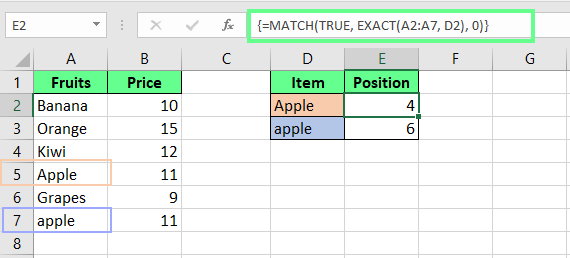
Combine EXACT() and MATCH(). Image by Author.

Final Thoughts

MATCH(), wildcards, and fuzzy matching may seem a bit tricky at first but with some practice, they can save us loads of time. They’re especially helpful when we work with messy data or need more flexible ways to find things in a spreadsheet.

If you want to explore more, our Data Analysis in Excel course is a great next step. Or check out our Excel Fundamentals skill track to build up your basics and feel more confident using functions like these.

You may make mistakes initially but don’t stress if it takes a few attempts. It’s all part of getting comfortable with Excel.