Excel UNIQUE(): The Fastest Way to Filter Duplicates

Excel’s UNIQUE() function takes any hassle out of what can be an annoying process of de-duping data. It’s a simple formula, but it’s a must-know because, as you will see in this article, it can extract distinct entries from any range, no matter how long the list (within reason) or how often it changes. In this article, you will see clear examples and ready-to-use code blocks that you can just copy and paste into your worksheet, with small changes, and I hope you find it helpful. 

What Does the Excel UNIQUE() Function Do?

Let’s start with the main idea. UNIQUE() returns a list of unique values from a range or array, automatically filling as many cells as needed. This is known as a dynamic array. 

This makes it good for instantly stripping duplicates from a column or generating fresh lists for dropdown menus or reports.

As a quick heads up, UNIQUE() is available only in Excel for Microsoft 365, Excel 2021, and Excel for the web. If you’re using an older version, you’ll need an alternative, which I’ll also show later on.

Excel UNIQUE() Function Syntax

We now know what it does so I’ll show you the syntax:

=UNIQUE(array, [by_col], [exactly_once])

Here’s what each argument means:

• array: The range or array from which you want to extract unique values.

• by_col (optional): Set this to TRUE to compare columns instead of rows. Most of the time, you’ll leave it blank or set to FALSE.

• exactly_once (optional): Set to TRUE if you want only values that appear once in the source array. By default (FALSE), you’ll get all distinct values, even if they appear more than once.

In the next sections, when we practice examples, you will see these arguments in action.

Excel UNIQUE() for Values in a List

Suppose you have a list of cities in column A (A2 to A10), and some cities are listed more than once. To pull out just the unique city names, enter this:

=UNIQUE(A2:A10)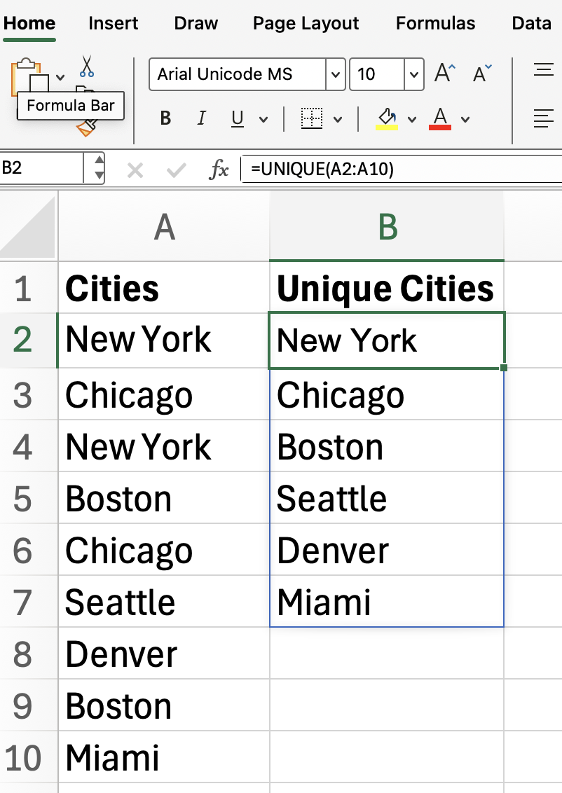

Excel will “spill” the unique city names down the column, starting from the cell where you typed the formula. As long as the function is there, our list will update as your source data changes, which itself is another big time saver. If your list will grow in size, you might want to make your range extra long in anticipation of that.

Excel UNIQUE() Across Multiple Columns

Now what if your data spans more than one column? Let’s say you have a two-column table (A2:B10) with names and departments, and you want to see each unique name/department pair only once. This is a lesser-known ability of the function, and well worth knowing. 

=UNIQUE(A2:B10)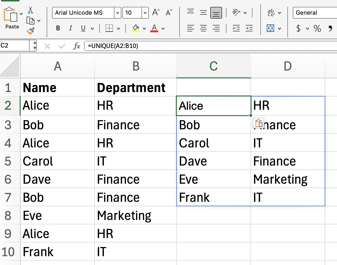

With this formula, Excel returns each unique combination of name and department, eliminating duplicate rows. If you only care about unique names, you can point UNIQUE() directly to just the name column, which is like what we showed earlier.

=UNIQUE(A2:A10)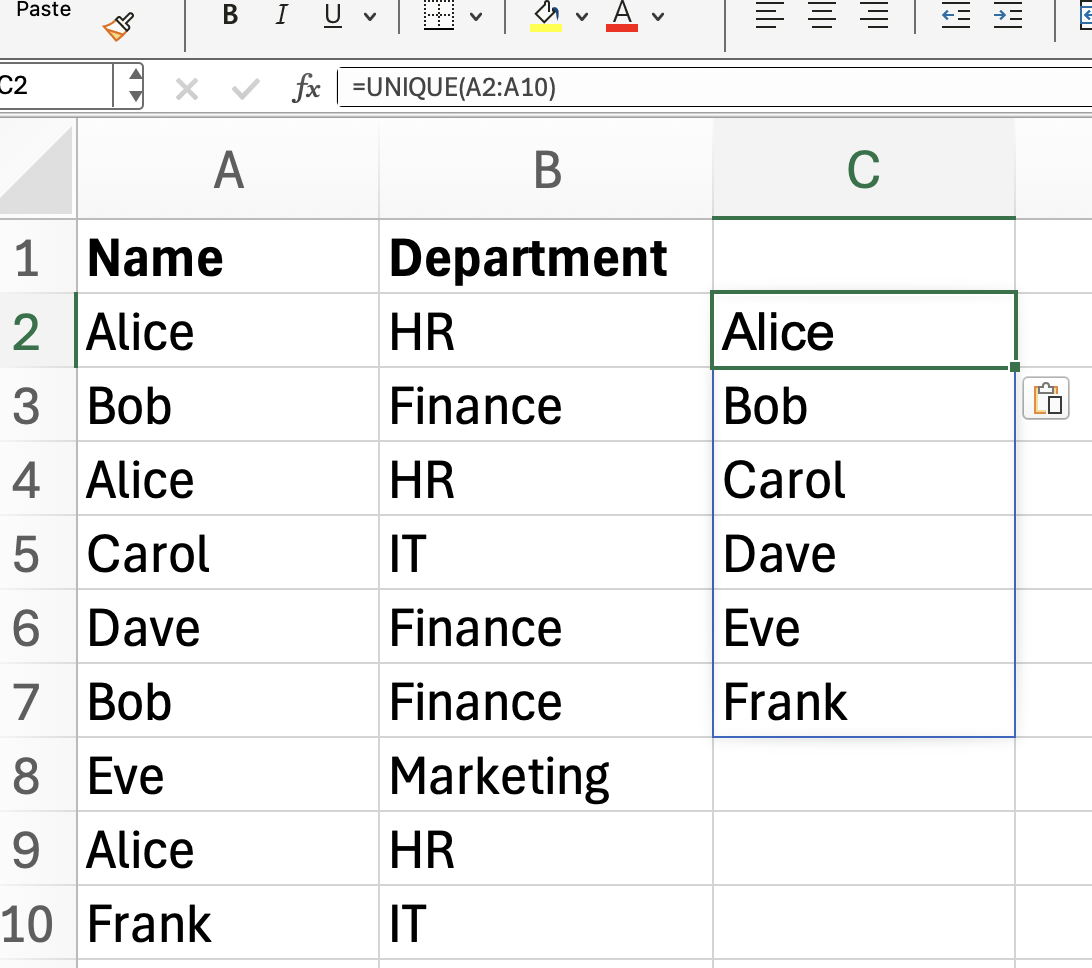

Excel UNIQUE() to Show Values That Appear Exactly Once

As we saw before, UNIQUE() by default gives you all distinct values, even if they appear more than once. But you can actually use UNIQUE() to filter out any value that’s repeated, showing only those that appear exactly once. (I showed the function syntax earlier for a reason.) For this next example, we will use the exactly_once argument.

=UNIQUE(A2:A10, FALSE, TRUE)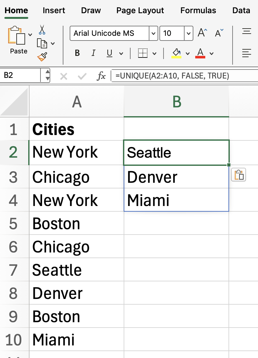

This formula returns only the values from A2:A10 that occur a single time, so we can spot those one-off entries. Notice how New York, Chicago, and Boston is not included. 

Excel UNIQUE() to Get Unique Columns Instead of Rows

So far, we’ve focused on extracting unique rows, but UNIQUE() can also help you find unique columns. If you set by_col to TRUE, Excel flips the usual behavior and compares columns across the specified range and returns just the distinct ones. I admit this is less common, but it can be useful in certain scenarios.

=UNIQUE(A1:F1, TRUE)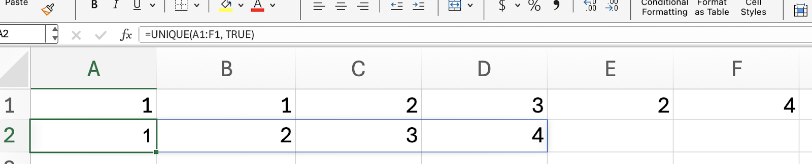

Here, Excel checks each column within the selected range and gives you only the columns that are different from one another. 

Excel UNIQUE() with Other Functions

Now that you’re comfortable with UNIQUE() by itself, let’s see how it works with other dynamic array functions. 

To sort your unique values alphabetically, simply wrap the UNIQUE() function in SORT():

=SORT(UNIQUE(A2:A10))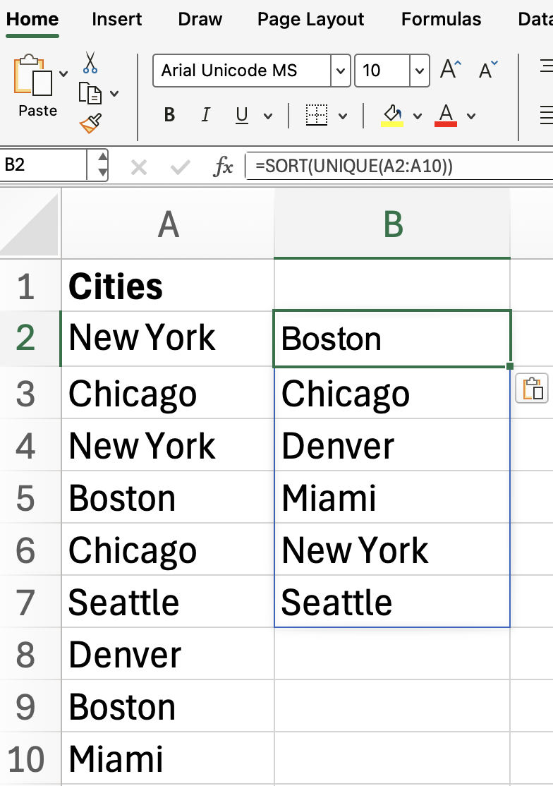

Or, if you want to extract unique values based on a specific condition (say, only for "Active" entries), combine UNIQUE() with FILTER(). (And here’s another array formula, if you wanted more practice.)

=UNIQUE(FILTER(A2:A10, B2:B10="Active"))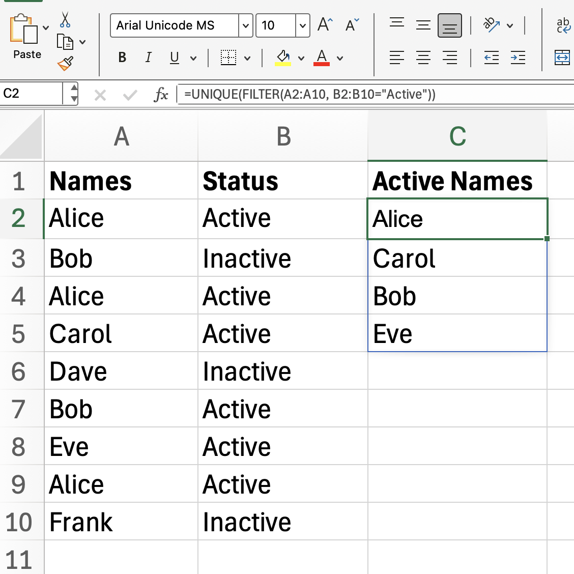

This formula returns only the unique items from A2:A10 where the corresponding row in B2:B10 is marked as “Active.” 

Alternatives to Excel UNIQUE()

You might be wondering how people managed before UNIQUE() arrived. Previously, extracting unique values involved longer formulas like this one, that I won’t finish all the way:

=IFERROR(INDEX(...

Or else, if you didn’t know of UNIQUE(), you might go through an arduous process of manually removing duplicates, or else you might use PivotTables as anothe common method. 

These methods still work, and might be the option for older Excel versions, but if you’re using a newer version, try UNIQUE() instead because it’s definitely more efficient.

Excel UNIQUE() Common Issues

As a final section, I’ll point out some common issues, in case you encounter them:

• The results “spill” into as many rows or columns as needed. If you type in any of these cells, you’ll get a #SPILL! error—so keep those cells clear.

• UNIQUE() is case-insensitive, treating “Apple” and “apple” as the same.

• If your source range updates, the UNIQUE() output updates automatically, keeping your data fresh.

Conclusion

Excel’s UNIQUE() function is what you use when you need to clean up data, create dropdowns, or summarize info with less effort than writing another formula. We also practiced how to use UNIQUE() with other functions such as SORT() and FILTER(). Take our Advanced Excel Functions course to learn even more, such as lookup functions and database functions.