PivotTable Conditional Formatting: Two Good Methods

Applying conditional formatting to PivotTables adds value to our data analysis by visually highlighting the most critical data points and enhancing the readability of those tables.

In this tutorial, we'll learn two methods for applying conditional formatting to PivotTables in Excel. We'll also list some nuances and potential issues to keep in mind and how to handle them.

If you need a quick revision of the basics of Excel, our Introduction to Excel course can be a helpful resource for you.

How to Apply Conditional Formatting to PivotTables

There are two methods for applying conditional formatting to PivotTables in Excel:

• Choosing from the predefined rule types and formats
• Using a dedicated rule manager.

Both methods start with:

• Selecting one of the cells to which we want to apply conditional formatting,
• Opening the Home tab on the Excel ribbon
• Clicking on the Conditional Formatting button.

The first method is more intuitive and provides preset formats for each rule. The second method is a little more customizable and allows accessing all options, settings, and already-created rules from one place.

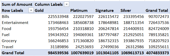
To practice both methods, in this tutorial, we're going to work with the below PivotTable based on the source table from Kaggle—Credit Card Spending Habits in India:

Method 1: Using the PivotTable formatting icon

Let's see how to implement the first method: choosing from the predefined rule types, rules, and formats.

• Select one of the cells of interest in your PivotTable.
• Open the Home tab on the Excel ribbon.
• Click on the Conditional Formatting button.
• Choose the predefined options:
• Select one of the rule types in bold.
• Follow the steps that appear to select a rule and a format.
• Click on the Formatting Options icon that appears to the right of the cell.

You can customize things like the rule type, condition (e.g., greater than or top 10), font color, cell fill color, number formatting, and even icon sets.

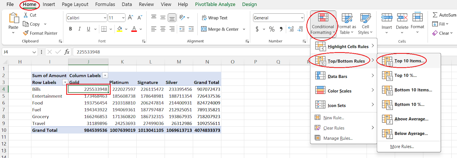
Choosing from the predefined conditional formatting rules. Image by Author

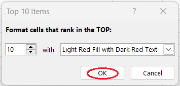
Choosing from the predefined formats. Image by Author

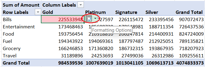
Opening the formatting options. Image by Author

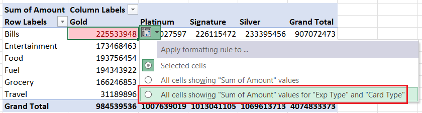
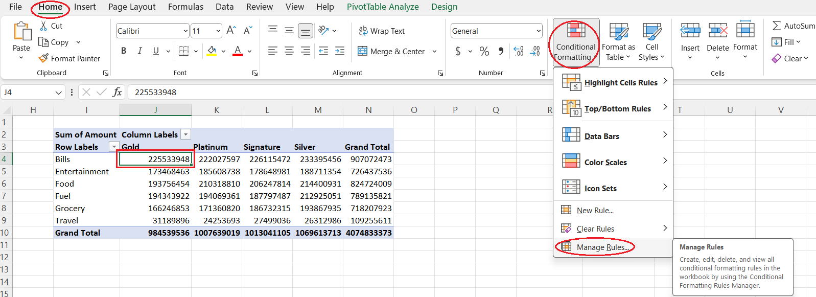
Expanding a conditional formatting rule to all cells. Image by Author

Method 2: Using the Conditional Formatting rules manager

Now, let’s practice applying conditional formatting to our PivotTable by using the second method: setting a rule type, a rule, and a format in a dedicated rule manager.

• Select one of the cells of interest in your PivotTable.
• Open the Home tab on the Excel ribbon.
• Click on the Conditional Formatting button.
• Use a dedicated rule manager:
• Select Manage Rules.
• Click on the New Rule button.
• Select the third option for the Apply Rule To: section.
• Select a rule type.
• Manually set the format.

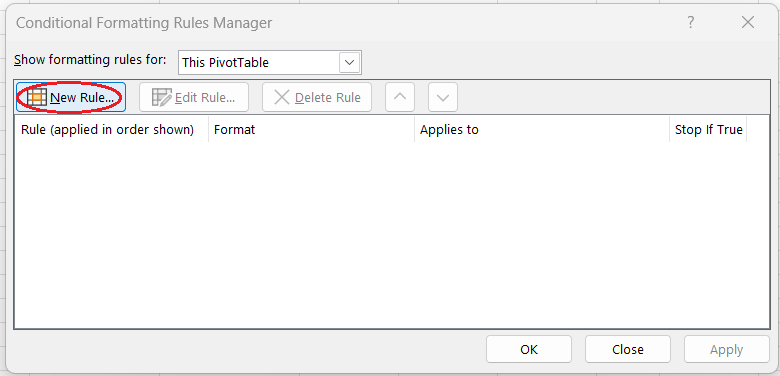
Opening the Conditional Formatting Rules Manager. Image by Author

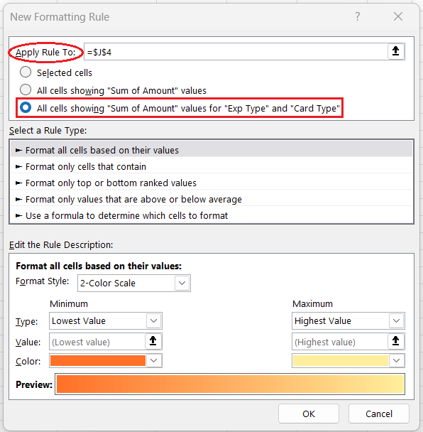
Creating a new rule in the Conditional Formatting Rules Manager. Image by Author

Expanding a conditional formatting rule to all cells. Image by Author

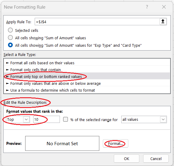
Selecting a rule type, building a rule, and opening the format constructor. Image by Author

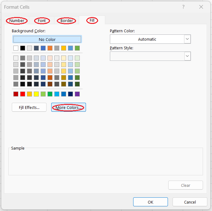
Setting format details. Image by Author

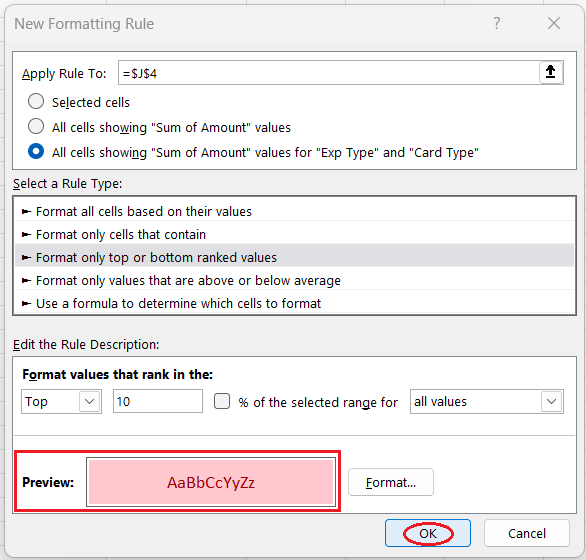
Confirming the creation of a new rule. Image by Author

Things To Keep in Mind

1. Conditional formatting is applied directly to the PivotTable. We don't need to apply any conditional formatting to the original Excel table on which our PivotTable is based.
2. If you change anything to the underlying table, it's necessary to refresh the PivotTable to make sure the conditional formatting is applied to it.
3. Conditional formatting rules remain valid and work as expected after rearranging the PivotTable layout or applying filters or slicers.
4. Conditional formatting is lost if we remove from the PivotTable any of the fields to which that formatting was applied.

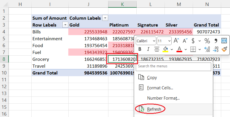
Refreshing a PivotTable with conditional formatting after updating the source table. Image by Author

Conclusion

Now it's your turn to practice and experiment with different conditional formatting techniques that can work better in other cases. Our Data Analysis in Excel course is a great place to continue mastering your skills.