Using TensorFlow 2.0 to Compose Music Tutorial

This tutorial was developed around TensorFlow 2.0 in Python, along with the high-level Keras API, which plays an enhanced role in TensorFlow 2.0. For those who would like to learn more about TensorFlow 2.0, see Introduction to TensorFlow in Python on DataCamp. For an exhaustive review of the deep learning for music literature, see Briot, Hadjerest, and Pachet (2019), which we will refer to throughout this tutorial.

Generative Models

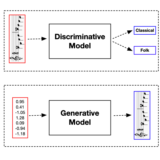
Supervised machine learning models can be divided into two categories: discriminative models and generative models. Discriminative models identify a decision boundary and produce a corresponding classification. Generative models create new instances of a class.

A discriminative model of music could be used to classify songs into different genres. A generative model might compose songs of a particular genre. In this tutorial, we'll make use of generative models to compose music.

Music Representation

Before we can define and train a generative model, we must first assemble a dataset. For music, data can be represented using either a continuous or discrete form. The most common continuous form is an audio signal, typically stored as a WAV file. We will not use continuous forms in this tutorial, but you can read more about them in the Appendix. Common discrete forms include Musical Instrument Digital Interface (MIDI) files, pianoroll, and text. We will focus on MIDI files and will extract two types of symbolic objects: notes and chords.

Notes

A note is a symbolic representation of a sound. For our purposes, a note can be described by its pitch and duration. A note's pitch is related to the frequency of oscillation of its sound wave, which is measured in hertz (Hz). Notes with higher pitches have sound waves with more oscillations per second. A note's duration is the length of the period over which it is played.

MIDI files represent a note's pitch with an integer between 0 and 127. Notes may also be represented by a pitch letter and octave number. Within the same octave, the pitches are ordered from lowest to highest frequency as follows:

1. C
2. C#/D♭
3. D
4. E♭/D#
5. E
6. F
7. F#/G♭
8. G
9. A♭/G#
10. A
11. B♭/A#
12. B

The octave is indicated by a subscript, such as the 4 in A₄ or the 7 in C₇. A higher octave corresponds to a higher frequency. If we take an arbitrary pitch, X_i, then the pitch X_i+1, which is exactly one octave higher, represents a sound wave with twice the frequency of X_i.

In addition to a note's pitch, we will also make use of its duration. The duration is a relative value, which is normalized by the length of a whole note. The longest note is a "large" note, which is eight times as long as a whole note. The shortest note is a two hundred fifty-sixth note, which is 1/256th the length of a whole note.

Chords

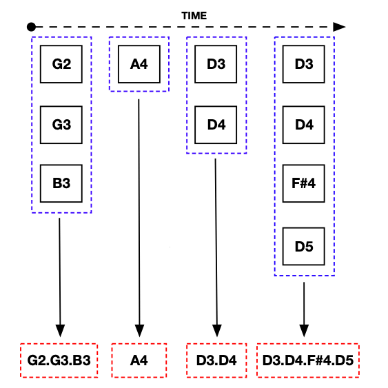
A chord is a combination of two or more notes played simultaneously on the same instrument. If we look at monophonic music -- that is, music played on a single instrument -- we may identify chords by assuming that all notes played at the exact same time are part of the same chord. This assumption is not valid if we have polyphonic music, which consists of two or more instruments playing simultaneously.

In the code block below, we install music21 and then import the converter module, which we will use to parse MIDI files. We will load and parse a classical guitar piece by Mauro Giuliani. We will then apply the .chordify() method, which reconstructs the sequence of chords in the score, assuming that notes played simultaneously are part of the same chord.

!pip install music21
from music21 import converter

# Define data directory
data_dir = '../audio/'

# Parse MIDI file and convert notes to chords
score = converter.parse(data_dir+'giuliani.mid').chordify()

# Display as sheet music
print(score.show())

After constructing the sequence of chords in the MIDI file, we can display it as sheet music using the .show() method. This will require the use of software that can create and display sheet music, such as MuseScore, which is available for free.

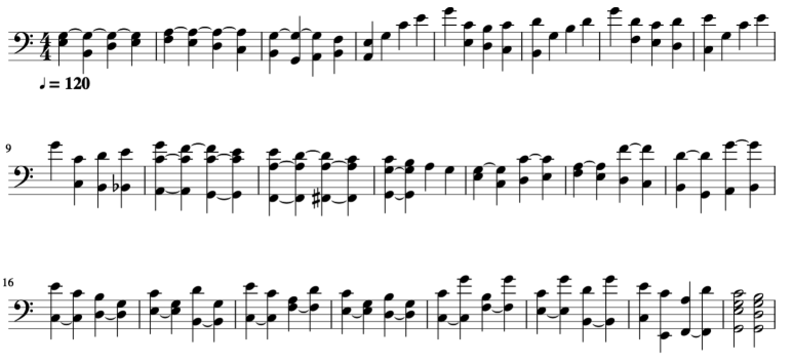
Alternatively, we may wish to examine and manipulate the underlying elements as text. We can do this using the .show('text') method. At the start of each line, we can see the offset in brackets, which tells us how many seconds into the score an element appears. Notice that only one of the elements at the 0th second is a chord. The rest of the elements are metadata, including the instrument used, the tempo, the key, and the meter. We will make use of the key later, but you can ignore these elements for now.

 print(score.show('text'))
{0.0} <music21.instrument.Guitar 'Guitar'>
{0.0} <music21.tempo.MetronomeMark animato Quarter=120.0>
{0.0} <music21.key.Key of C major>
{0.0} <music21.meter.TimeSignature 4/4>
{0.0} <music21.chord.Chord E3 G3>
{1.0} <music21.chord.Chord B2 G3>
{2.0} <music21.chord.Chord D3 G3>
...
{46.0} <music21.chord.Chord A3>
...
{88.0} <music21.chord.Chord G2 E3 G3 C4>
{90.0} <music21.chord.Chord G2 D3 G3 B3>
{92.0} <music21.chord.Chord C3 E3 G3 C4>

After the metadata, the remaining elements consist of chords, ordered in the sequence in which they appear in the song. For instance, <music21.chord.Chord E3 G3> is the chord produced by playing notes E₃ and G₃. Additionally, <music21.chord.Chord A3> is the note A₃ played in isolation.

For some models, we will use both the chord and its duration, which measures the amount of time it is played. We can get this information by applying the .elements methods and accessing the .duration attribute for an arbitrary chord in the score, as shown in the code block below.

print(score.elements[10])
<music21.chord.Chord E3 A3>
print(score.elements[10].duration)
<music21.duration.Duration 1.0>

Note and Chord Encoding

Throughout this tutorial, we will focus on discrete representations of music that can be described by sequences of notes, chords, and associated durations. Recall that chords are combinations of notes and that the MIDI format permits the use of 128 individual notes. If we want to expand the feature set to include all two-note chords, this increases its size by 128!/[(128-2)!*2!] or 8128 elements. Adding three-note chords expands this by 341,376, and adding four-note chords expands this by another 10,668,000.

The example we showed earlier contains notes and two-note, three-note, and four-note chords. If we use one-hot encoding and include all features, we will need to make predictions over 11,017,632-dimensional vectors. Consequently, we will want to think carefully about our choice of encoding in music generation problems. We may also want to consider using key transposition or data augmentation, both of which are discussed in the Appendix.

With respect to the choice of encoding, Briot, Hadjerest, and Pachet (2019) discuss four different options that are commonly used in generative models of music:

1. One-Hot Encoding
2. Many-Hot Encoding
3. Multi-One-Hot Encoding
4. Multi-Many-One-Hot Encoding

One-hot encoding represents musical symbols, such as notes and chords, as sparse vectors with a one in the position that corresponds to a particular note or chord. Many-hot encoding represents chords, which consist of multiple notes, by placing a one in the position that corresponds to each of the notes.

In the diagram below, we compare many-hot and one-hot encodings for the case where we have notes and two-note chords. With many-hot encodings, the notes C₄ and D₄ are represented by vectors with 128 elements. Both vectors have zeros in all positions other than the positions that correspond to the C₄ and D₄ elements, which contain ones. The C₄+D₄ chord, which is the product of playing notes C₄ and D₄ simultaneously, is constructed by placing ones in both the C₄ and D₄ positions.

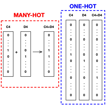
The one-hot representation of single notes and two-note chords consists of 8256-element vectors. In each case, a vector is sparse and contains a 1 in the position that corresponds to a unique note or chord. Notice that the many-hot representation requires the use of a multi-label model, where multiple classes may be predicted for a given output. It does, however, substantially reduce the size of the input and output vectors.

Most models in the literature still use one-hot encoding. However, Briot, Hadjerest, and Pachet (2019) identify several music generation models that make use of many-hot encoding, including the RBMc, RNN-RBM, and C-RBM systems, which are all based around a restricted Boltzmann machine (RBM) architecture.

Multi-one-hot encodings and multi-many-hot encodings are the generalizations of one-hot and many-hot encoding to the case where we have polyphonic music -- that is, multiple instruments playing simultaneously. We will restrict ourselves to monophonic music and will not discuss these options further in the tutorial.

Data Collection and Preparation

Our next step is to collect a dataset that we can use to train a generative model. We will make use of data from the Mutopia Project, which contains 2124 pieces of music in MIDI format that are in the public domain. Since the website is divided into sections by instrument, we can write a relatively simple Python script to scrape all of the guitar pieces, which we will use to train models in this tutorial. For an overview of how to do this, see the Appendix.

Let's assume we've saved all of the .mid files from the guitar section to a directory, save_dir. The next step is to load each .mid file into music21 as a stream object.

import os
from music21 import converter, pitch, interval

# Define save directory
save_dir = '../guitar/'

# Identify list of MIDI files
songList = os.listdir(save_dir)

# Create empty list for scores
originalScores = []

# Load and make list of stream objects
for song in songList:
    score = converter.parse(save_dir+song)
    originalScores.append(score)

As part of our dimensionality reduction strategy, we'll restrict ourselves to the songs composed by Mauro Giuliani. We can do this by modifying the code block above as follows.

# Identify list of MIDI files
songList = os.listdir(save_dir)
songList = [song for song in songList if song.lower().find('giuliani')>-1]

We need to do four additional things before we can begin training:

1. Remove polyphonic music and apply .chordify() to the remaining stream objects.
2. Extract the sequence of notes, chords, and durations.
3. Construct a mapping that translates notes, chords, and durations to integers and vice-versa.
4. Divide streams into sequences of fixed length that may be used as inputs to models.

Let's start by removing polyphonic music from the dataset. We can do this by partitioning each stream object by instrument and then checking whether there is only one partition -- that is, whether only one instrument is playing. We will do that in the code block below.

from music21 import instrument

# Define function to test whether stream is monotonic
def monophonic(stream):
    try:
        length = len(instrument.partitionByInstrument(stream).parts)
    except:
        length = 0
    return length == 1

# Merge notes into chords
originalScores = [song.chordify() for song in originalScores]

Note that if we apply .chordify() -- depicted in the figure below -- without removing polyphonic music, we will accidentally merge notes played by different instruments into a chord.

We now need to extract notes, chords, and durations from each stream. We'll first define three empty lists: originalChords, originalDurations, originalKeys. We can enumerate over the list of streams. For each stream, we'll identify and store all notes, chords, and durations, as well as the piece's key.

from music21 import note, chord

# Define empty lists of lists
originalChords = [[] for _ in originalScores]
originalDurations = [[] for _ in originalScores]
originalKeys = []

# Extract notes, chords, durations, and keys
for i, song in enumerate(originalScores):
    originalKeys.append(str(song.analyze('key')))
    for element in song:
        if isinstance(element, note.Note):
            originalChords[i].append(element.pitch)
            originalDurations[i].append(element.duration.quarterLength)
        elif isinstance(element, chord.Chord):
            originalChords[i].append('.'.join(str(n) for n in element.pitches))
            originalDurations[i].append(element.duration.quarterLength)
    print(str(i))

We'll perform further dimensionality reduction in the code block below by retaining only music with the C major key signature, which happens to be the most common in our dataset. We will also use the word "chord" to refer to both chords and notes in the remainder of the tutorial.

# Create list of chords and durations from songs in C major
cMajorChords = [c for (c, k) in zip(originalChords, originalKeys) if (k == 'C major')]
cMajorDurations = [c for (c, k) in zip(originalDurations, originalKeys) if (k == 'C major')]

The next step is to identify the unique set of chords and durations. We will then construct dictionaries that map them to integers. If we print the number of unique notes and chords, we can see that the dimensionality reduction steps we've taken have lowered the number to a manageable 267.

# Map unique chords to integers
uniqueChords = np.unique([i for s in originalChords for i in s])
chordToInt = dict(zip(uniqueChords, list(range(0, len(uniqueChords)))))

# Map unique durations to integers
uniqueDurations = np.unique([i for s in originalDurations for i in s])
durationToInt = dict(zip(uniqueDurations, list(range(0, len(uniqueDurations)))))

# Print number of unique notes and chords
print(len(uniqueChords))
267

# Print number of unique durations
print(len(uniqueDurations))
9

After we've trained our model and made predictions, we will want to map our integer predictions back to notes, chords, and durations. We'll invert the chordToInt and durationToInt dictionaries below.

# Invert chord and duration dictionaries
intToChord = {i: c for c, i in chordToInt.items()}
intToDuration = {i: c for c, i in durationToInt.items()}

Finally, we can define our training sequences, which consist of 32 consecutive notes and chords, along with their corresponding durations. We will first do this for autoencoder-type models, where our set of features and targets are the same.

# Define sequence length
sequenceLength = 32

# Define empty arrays for train data
trainChords = []
trainDurations = []

# Construct training sequences for chords and durations
for s in range(len(cMajorChords)):
    chordList = [chordToInt[c] for c in cMajorChords[s]]
    durationList = [durationToInt[d] for d in cMajorDurations[s]]
    for i in range(len(chordList) - sequenceLength):
        trainChords.append(chordList[i:i+sequenceLength])
        trainDurations.append(durationList[i:i+sequenceLength])

Music Generation

In this section, we'll make use of the dataset we assembled and prepared to generate music. We'll consider three different models of music generation, starting with the simplest:

1. The Autoencoder
2. The Variational Autoencoder (VAE)
3. The Long Short-Term Memory Model (LSTM)

Autoencoders

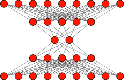
An autoencoder consists of two networks, which are stacked-vertically and joined by a latent vector. The inputs to an autoencoder are first passed to an encoder model, which typically consists of one or more dense layers. The final layer in the encoder model is called a latent vector. This is a bottleneck that forces the features extracted in the encoder to be compressed into a small number of latent features.

The latent vector connects to a decoder model, which upsamples or decompresses the data. The number of nodes in each successive decoder layer increases. The final output layer has the same dimensions as the input layer of the encoder model.

In contrast to discriminative models, which attempt to identify a decision boundary, autoencoders are trained to reconstruct the input data -- in this case, a song -- as accurately as is possible, subject to the constraints placed by the size of the latent vector. For this reason, autoencoders simply use the inputs as the target.

We'll use an autoencoder to construct our first generative model of music. To keep things as simple as is possible, we'll adopt the architecture for the MiniBach model introduced in Briot, Hadjerest, and Pachet (2019) as a simplification to the DeepBach model. For another example of an autoencoder model of music generation, see the DeepHear system.

The input data, as we've constructed it, consists of one-hot encoded vectors that represent notes and chords. We will ignore durations for now. Following the MiniBach architecture, we'll start by flattening the input vector.

# Convert to one-hot encoding and swap chord and sequence dimensions
trainChords = tf.keras.utils.to_categorical(trainChords).transpose(0,2,1)

# Convert data to numpy array of type float
trainChords = np.array(trainChords, np.float)

# Flatten sequence of chords into single dimension
trainChordsFlat = trainChords.reshape(nSamples, nChordsSequence)

We next define the number of samples, nSamples, the number of chords and notes, nChords, and the size of the input dimension, inputDim. We also set the number of latent features, latentDim, to 2. Using a low number of latent dimensions will reduce performance, but it will allow us to easily generate visualizations of the latent space.

# Define number of samples, chords and notes, and input dimension
nSamples = trainChords.shape[0]
nChords = trainChords.shape[1]
inputDim = nChords * sequenceLength

# Set number of latent features
latentDim = 2

We now define the architecture for the model, starting with the input layer for the encoder network, encoderInput, and the input layer for the decoder network, latent. Note that the latent layer is also the output of the encoder network. We next define a dense layer, encoded, that connects the inputs to the latent vector and another dense layer, decoded, which connects the latent vector to the output vector.

Finally, we define a decoder model, decoder, and our autoencoder, autoencoder. Note that .Model() has an inputs and outputs argument. For the decoder model, we pass the latent vector as an input and the decoded network as an output. For the full autoencoder, we use encoderInput as the input and pass the the decoder model, evaluated using the output of the encoder network, encoded, as an input.

# Define encoder input shape
encoderInput = tf.keras.layers.Input(shape = (inputDim))

# Define decoder input shape
latent = tf.keras.layers.Input(shape = (latentDim))

# Define dense encoding layer connecting input to latent vector
encoded = tf.keras.layers.Dense(latentDim, activation = 'tanh')(encoderInput)

# Define dense decoding layer connecting latent vector to output
decoded = tf.keras.layers.Dense(inputDim, activation = 'sigmoid')(latent)

# Define the encoder and decoder models
encoder = tf.keras.Model(encoderInput, encoded)
decoder = tf.keras.Model(latent, decoded)

# Define autoencoder model
autoencoder = tf.keras.Model(encoderInput, decoder(encoded))

The architecture for a generic autoencoder is shown in the figure below. The top half of the network is the encoder, and the bottom half is the decoder. They are connected by the latent vector.

With the architecture defined for the decoder and autoencoder, the only steps that remain are to compile the model and then train using the .fit() method. There are two important details to notice:

1. Our input values will consist of 0s and 1s, and our predicted values will be real numbers between 0 and 1. We can use a binary_crossentropy loss function.
2. Both the input values and targeted values are the same: trainChordsFlat.

# Compile autoencoder model
autoencoder.compile(loss = 'binary_crossentropy', learning_rate = 0.01, optimizer='rmsprop')

# Train autoencoder
autoencoder.fit(trainChordsFlat, trainChordsFlat, epochs = 500)

The last step is to generate music. Since we set the sequence length to 32, the autoencoder will take 32 chords and notes as inputs and produce a fixed-length "song" that consists of a sequence of 32 chords and notes. The autoencoder is trained to generate outputs that are highly similar to the input; however, our objective is to generate new music. To do this, we'll pass a randomly-generated latent vector to the decoder model, which we defined as a subnetwork of the autoencoder model.

# Generate chords from randomly generated latent vector
generatedChords = decoder(np.random.normal(size=(1,latentDim))).numpy().reshape(nChords, sequenceLength).argmax(0)

Notice that we reshaped the output of the autoencoder into an array with the same dimensions as our original input. We then took the argmax() over the first dimension of the array. This returns an integer value that corresponds to a chord, which we'll identify in the code block below.

# Identify chord sequence from integer sequence
chordSequence = [intToChord[c] for c in generatedChords]

Finally, we can create a stream object using music21, set the instrument as guitar, append the sequence of chords our model generated, and then export everything as a MIDI file.

# Set location to save generated music
generated_dir = '../generated/'

# Generate stream with guitar as instrument
generatedStream = stream.Stream()
generatedStream.append(instrument.Guitar())

# Append notes and chords to stream object
for j in range(len(chordSequence)):
    try:
        generatedStream.append(note.Note(chordSequence[j].replace('.', ' ')))
    except:
        generatedStream.append(chord.Chord(chordSequence[j].replace('.', ' ')))

generatedStream.write('midi', fp=generated_dir+'autoencoder.mid')

The gif below shows part of the training process for an autoencoder. The score generated in each step is the reconstruction associated with a specific latent state vector. Each frame represents 5 training epochs.

We can also visualize movement in the latent space during training, which we do in the gif below. Notice that the latent space is narrow and drifts across training epoch. This will make it difficult to draw a high-quality random latent state and will prove quite problematic when we use a higher dimensional latent vector. We will show in the next section how we can solve this using a variational autoencoder (VAE).

Finally, we may examine the audio output from our autoencoder. The chord sequence from the original song, which was drawn at random from our training set, is given first. We then generate a chord sequence from the autoencoder using the latent vector associated with the chord sequence from the original song, which yields the song below it.

Example: Original Song

Example: Generated Song

Variational Autoencoder

While autoencoders are well-suited to de-noising, compression, and decompression tasks, they do not perform well as generative models. Variational autoencoders (VAEs), introduced by Kingma and Welling (2017), are designed to overcome the weaknesses of autoencoders as generative models and are one of the most commonly-used methods for music generation. Briot, Hadjerest, and Pachet (2019) identify four different music-generation systems that are built on VAEs: MusicVAE, VRAE, VRASH, and GSLR-VAE. They improve on autoencoders along two dimensions:

1. Rather than mapping each set of inputs to a point in the latent space, a variational autoencoder maps each set of inputs to a normal distribution, characterized by a mean and a variance.
2. Rather than allowing the latent space to have any mean and variance, a variational autoencoder forces the mean and the natural logarithm of the variance to be close to 0.

We can make the first change by replacing the latent state vector in the autoencoder with three layers:

1. A mean layer
2. A (log) variance layer
3. A sampling layer

Each set of inputs maps to a single mean and the natural logarithm of the variance, which is sufficient to characterize a normal distribution. The model then randomly draws points from the distribution in the sampling layer.

The code block below defines a function that can be used to create a sampling layer. It takes a mean and log variance as inputs. It then uses the random submodule of tensorflow to draw a tensor of points, epsilon, from a standard normal distribution, which has both a mean and a log variance of 0. We next want to transform these draws into draws from distributions characterized by the mean and logVar parameters. To do this, we need to first scale the draws, epsilon, by the standard deviations of the associated distributions. We can compute these standard deviations by dividing logVar by 2 and then exponentiating it. We then add the distribution means, mean.

# Define function to generate sampling layer.
def sampling(params):
    mean, logVar = params
    batchSize = tf.shape(mean)[0]
    latentDim = tf.shape(mean)[1]
    epsilon = tf.random.normal(shape=(batchSize, latentDim))
    return mean + tf.exp(logVar / 2.0) * epsilon

We can now modify the autoencoder model to incorporate the mean, logVar, and sampling layers. Notice that the encoded layer now takes two inputs and the encoder layer has three outputs.

# Define the input and latent layer shapes.
encoderInput = tf.keras.layers.Input(shape = (inputDim))
latent = tf.keras.layers.Input(shape = (latentDim))

# Add mean and log variance layers.
mean = tf.keras.layers.Dense(latentDim)(encoderInput)
logVar = tf.keras.layers.Dense(latentDim)(encoderInput)

# Add sampling layer.
encoded = tf.keras.layers.Lambda(sampling, output_shape=(latentDim,))([mean, logVar])

# Define decoder layer.
decoded = tf.keras.layers.Dense(inputDim, activation = 'sigmoid')(latent)

# Define encoder and decoder layers.
encoder = tf.keras.Model(encoderInput, [mean, logVar, encoded])
decoder = tf.keras.Model(latent, decoded)

# Define variational autoencoder model.
vae = tf.keras.Model(encoderInput, decoder(encoded))

As was the case with the autoencoder model, our latent state is the output of the encoded layer. There is, however, an important difference: instead of mapping each set of inputs to a single latent state, we use the sampling layer to map them to random values drawn from a normal distribution with parameters mean and logVar. This means that the same input will be associated with a distribution of latent states.

The final step is to adjust the loss function to place discipline on the model's choice of mean and logVar values. In particular, we will compute the Kullback-Leibler (KL) divergence between each distribution defined by the mean and logVar layers, and the standard normal distribution, which has a mean and log variance of 0. The further our means and log variances are away from 0, the higher the KL divergence loss component will be.

A natural question is why we would want to force each distribution to be close to a standard normal. The reason we do this is that we want to sample latent states and use them to generate music. If we apply the KL divergence penalty to the loss function, this will allow us to use independent draws from a standard normal distribution to obtain latent states that are likely to generate high quality pieces of music.

In the code block below, we show how to modify the loss function to incorporate the KL divergence term. The first component of the loss function is the binary crossentropy loss, computed on the inputs to and outputs from the vae model. This is also what we used for the autoencoder. It is called a "reconstruction loss" because it penalizes us for failing to reconstruct the original song. The KL term is the mean KL divergence between the latent space distributions and the standard normal distribution. We combine the two to compute the total loss, vaeLoss, add that to the model, compile, and then train.

# Define the reconstruction loss.
reconstructionLoss = tf.keras.losses.binary_crossentropy(vae.inputs[0], vae.outputs[0])

# Define the Kullback-Liebler divergence term.
klLoss = -0.5 * tf.reduce_mean(1 + logVar - tf.square(mean) - tf.exp(logVar), axis = -1)

# Combine the reconstruction and KL loss terms.
vaeLoss = reconstructionLoss + klLoss

# Add the loss to the model.
vae.add_loss(vaeLoss)

# Compile the model.
vae.compile(batch_size = batchSize, learning_rate = 0.01, optimizer='rmsprop')

# Train the model.
vae.fit(trainChordsFlat, epochs = 500)

In the previous section, we showed that the latent space for the autoencoder was not well-behaved. Part of the purpose of a VAE is to overcome this design flaw in generative settings. The figure below shows the latent space for the VAE. We can see that there's a significant amount of dispersion across both features. Furthermore, they are both centered around 0 and do not drift across training epoch. This will make it much easier to randomly sample a high-quality latent state.

Finally, we move to music generation. We draw a random latent vector from the standard normal distribution, pass it to the decoder, reshape the output, and take the argmax of each column. This will return a sequence of 32 integers, which correspond to notes and chords, which we next identify using the intToChord dictionary. We then define a stream object, append guitar as the instrument, add the sequence of notes and chords to the stream, and then export it as a MIDI file.

# Generate integers from randomly drawn latent state.
generatedChords = decoder(np.random.normal(size=(1,latentDim))).numpy().reshape(nChords, sequenceLength).argmax(0)

# Identify chords associated with integers.
chordSequence = [intToChord[c] for c in generatedChords]

# Initialize stream with guitar as instrument.
generatedStream = stream.Stream()
generatedStream.append(instrument.Guitar())

# Append notes and chords and export to MIDI file
for j in range(len(chordSequence)):
    try:
        generatedStream.append(note.Note(chordSequence[j].replace('.', ' ')))
    except:
        generatedStream.append(chord.Chord(chordSequence[j].replace('.', ' ')))

generatedStream.write('midi', fp=generated_dir+'vae.mid')

The three songs below were generated by the model. The first two songs are based on latent states associated with chord sequences in the training set. The final song is a linear combination of the latent states of song #1 and song #2. Since the VAE forces the latent space to be well-behaved, we can be reasonably certain that a linear combination of latent states will yield a high-quality latent state.

Example: Generated Song #1

Example: Generated Song #2

Example: Linear Combination of Song #1 and #2

One thing we can observe from the autoencoder and VAE-based music is that it lacks a strong melody. We can improve on this by adding more layers to the model and increasing the size of the training set. Alternatively, we can make use of a model that is designed to process sequential data, as we'll do in the following section.

Long Short-Term Memory (LSTM)

The final model we'll consider is the long short-term memory model (LSTM). This is a type of recurrent neural network (RNN) that has been modified to prevent the vanishing gradient problem. Briot, Hadjerest, and Pachet (2019) find that recurrent models are the most commonly used for the purpose of music generation. They identify more than 20 music generation systems that rely on an RNN or LSTM model, including BachBot, DeepBach, Performance-RNN, and Hexahedria.

Using an LSTM model offers two benefits over an autoencoder-based model:

1. They are designed to process sequential data.
2. They can generate musical sequences of any length.

Unlike autoencoders and VAEs, which use the inputs as the targets, LSTM-based generative music models are instead trained to make a prediction about the next note or chord in the sequence. For this reason, we will need to reconstruct our train and target sets, which we'll do in the code block below. Since using an LSTM model will also reduce the number of parameters we need to train, we'll add durations to the model, too.

# Set sequence length
sequenceLength = 32

# Define empty array for train data
trainChords = []
trainDurations = []
targetChords = []
targetDurations = []

# Construct train and target sequences for chords and durations
for s in range(len(cMajorChords)):
    chordList = [chordToInt[c] for c in cMajorChords[s]]
    durationList = [durationToInt[d] for d in cMajorDurations[s]]
    for i in range(len(chordList) - sequenceLength):
        trainChords.append(chordList[i:i+sequenceLength])
        trainDurations.append(durationList[i:i+sequenceLength])
        targetChords.append(chordList[i+1])
        targetDurations.append(durationList[i+1])

Note that trainChords and trainDurations are defined in the same way as they were earlier in the tutorial. We have only added targetChords and targetDurations, which consist of the chord and duration that follow the chords and durations in the train sequence. We next set the number of samples, chords, and durations, as well as the input dimension. We will also use separate embedding layers for chords and durations.

# Define number of samples, notes and chords, and durations
nSamples = trainChords.shape[0]
nChords = trainChords.shape[1]
nDurations = trainDurations.shape[1]

# Set the input dimension
inputDim = nChords * sequenceLength

# Set the embedding layer dimension
embedDim = 64

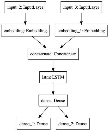
The next step is to define the model architecture. We will use a model with two inputs and two outputs, so that we can predict both chords and durations. We first define the input layers, chordInput and durationInput, and then pass these layers to embedding layers, chordEmbedding and durationEmbedding. These are look-up tables that associate a 64-element vector with each chord or duration. Embeddings allow us to replace a sparse vector representation, where inputs are one-hot encoded, with a dense representation, where related notes and durations have values that are closer to each other.

The outputs of the two embeddings layers are concatenated in mergeLayer. We then pass the output of this layer to two LSTM layers. The first layer sets the return_sequences parameter value to True. If we leave this parameter as False, as is done by default, the LSTM cells will return only the final states and not the intermediate sequential states. Recent work has shown that making use of intermediate states can improve performance. This is often done in the context of an attention layer. Finally, we pass the output of the LSTM layer to a dense layer, which is then passed to two output layers: chordOutput and durationOutput. We then define a keras functional API model by specifying the two input and two output layers.

# Define input layers
chordInput = tf.keras.layers.Input(shape = (None,))
durationInput = tf.keras.layers.Input(shape = (None,))

# Define embedding layers
chordEmbedding = tf.keras.layers.Embedding(nChords, embedDim, input_length = sequenceLength)(chordInput)
durationEmbedding = tf.keras.layers.Embedding(nDurations, embedDim, input_length = sequenceLength)(durationInput)

# Merge embedding layers using a concatenation layer
mergeLayer = tf.keras.layers.Concatenate(axis=1)([chordEmbedding, durationEmbedding])

# Define LSTM layer
lstmLayer = tf.keras.layers.LSTM(512, return_sequences=True)(mergeLayer)

# Define dense layer
denseLayer = tf.keras.layers.Dense(256)(lstmLayer)

# Define output layers
chordOutput = tf.keras.layers.Dense(nChords, activation = 'softmax')(denseLayer)
durationOutput = tf.keras.layers.Dense(nDurations, activation = 'softmax')(denseLayer)

# Define model
lstm = tf.keras.Model(inputs = [chordInput, durationInput], outputs = [chordOutput, durationOutput])

With the model defined, we can now compile and begin training. We have attempted to keep things as simple as is possible here, but for many applications, it will make sense to include regularization layers and additional dense and LSTM layers. Notice that the model has two input and two output layers, as is shown in the diagram below. You can learn more about models with multiple inputs and outputs in Introduction to TensorFlow in Python.

# Compile the model
lstm.compile(loss='categorical_crossentropy', optimizer='rmsprop')

# Train the model
lstm.fit([trainChords, trainDurations], [targetChords, targetDurations],
            epochs=500, batch_size=64)

Once the training process is complete, we can generate new songs using the LSTM model. We will do this by feeding in an initial sequence of 32 chords and durations, which will allow us to make our first predictions. We will then append those predictions to the chord and duration series, allowing us to make another prediction, based on the last 32 chords and durations of the updated series. One benefit of using an LSTM model is that we can iterate indefinitely, allowing us to generate songs of arbitrarily long length.

# Define initial chord and duration sequences
initialChords = np.expand_dims(trainChords[0,:].copy(), 0)
initialDurations = np.expand_dims(trainDurations[0,:].copy(), 0)

# Define function to predict chords and durations
def predictChords(chordSequence, durationSequence):
    predictedChords, predictedDurations = model.predict(model.predict([chordSequence, durationSequence]))
    return np.argmax(predictedChords), np.argmax(predictedDurations)

# Define empty lists for generated chords and durations
newChords, newDurations = [], []

# Generate chords and durations using 500 rounds of prediction
for j in range(500):
    newChord, newDuration = predictChords(initialChords, initialDurations)
    newChords.append(newChord)
    newDurations.append(newDuration)
    initialChords[0][:-1] = initialChords[0][1:]
    initialChords[0][-1] = newChord
    initialDurations[0][:-1] = initialDurations[0][1:]
    initialDurations[0][-1] = newDuration

The final step is to export the generated music to a MIDI file using music21. Note that the code is nearly identical to what we used for the autoencoder-based models, but with one important difference: we are now appending both chords and durations to the stream object.

# Create stream object and add guitar as instrument
generatedStream = stream.Stream()
generatedStream.append(instrument.Guitar())

# Add notes and durations to stream
for j in range(len(chordSequence)):
    try:
        generatedStream.append(note.Note(chordSequence[j].replace('.', ' '), quarterType = durationSequence[j]))
    except:
        generatedStream.append(chord.Chord(chordSequence[j].replace('.', ' '), quarterType = durationSequence[j]))

# Export as MIDI file
generatedStream.write('midi', fp=generated_dir+'lstm.mid')

With the autoencoder and VAE models, we struggled to generate melodies and could only output fixed-length songs. Using an LSTM model, we can generate output sequences of arbitrary lengths by iterating over predictions, as we've done in the code block above. It will also be relatively easier to generate better melodies. We will see both of these features in the examples below, each of which is seeded with an initial sequence of chords and durations from a sample in our training set.

Example: Generated Song #1

Example: Generated Song #2

Example: Generated Song #3

Additional Issues

Data

One of the major challenges to the development of machine learning models for music is the availability of datasets, since music is typically not freely and legally available for download. In fact, this has prevented the literature from coordinating on a standard practice dataset, such as the MNIST dataset for image classification. There are, however, a few projects which provide either raw audio, symbolic notation, or derived musical features for a large number of songs. We provide a partial list of those projects below.

1. Mutopia Project. An archive of public domain and creative commons music in MIDI, PDF, and LilyPond formats. It currently contains over 2000 songs and is organized by instrument, composer, style, and collection.
2. The Million Song Dataset. Contains audio features and metadata for over 300gb worth of popular music tracks, but no audio tracks.
3. Free Music Archive. Contains audio, genre labels, and features for over 100,000 tracks that are freely and legally available for download.

Sampling vs Determinism

When we generated music using an LSTM model, we used a deterministic approach to the selection of chords and durations. The model predicted probabilities for each of the 267 chords and 9 durations, and we selected the chords and durations with the highest associated probabilities. Similarly, for the autoencoder and variational autoencoder models, we selected the chords with the highest associated output values.

One alternative to this approach is to sample from the distribution of outputs, rather than selecting the chords and durations with the highest probabilities. This will make the music generation process stochastic, rather than deterministic. This means that autoencoder or VAE models with the same latent vector will generate different songs each time they are run. Similarly, the same sequence of inputs to an LSTM model will be able to generate different songs.

The code block below shows how we can move to stochastic chord and duration generation by modifying the predictChords() function. Note that we have replaced the argmax() operation with a sampling operation that uses the probabilities to perform random draws from the vectors of chords and durations.

# Define function to generate chords and durations stochastically
def predictChords(chordSequence, durationSequence):
    predictedChords, predictedDurations = model.predict([chordSequence, durationSequence])
    return np.random.choice(range(nChords), p = predictedChords), np.random.choice(range(nDurations), p = predictedDurations)

For an extended discussion of the benefits of the stochastic and deterministic approaches to music generation, see section 6.6 of Briot, Hadjerest, and Pachet (2019).

Embeddings

When we trained the LSTM model, we used a layer of embeddings, which mapped each input chord and duration to a dense, 64-element vector. Using an embedding layer allows us to avoid using sparse, high-dimensional vectors as inputs. Instead, we use a low-dimensional representation that allows us to identify relationships between different chords.

In many cases, it will not make sense to train an embedding layer. This is because we will often not have sufficiently large training sets when working on music generation problems. Using pre-trained embeddings or embeddings produced using unsupervised learning -- as we often do for text classification and generation problems -- will allow us to train the model when it would otherwise be infeasible.

See Chuan, Agres, and Herremans (2018) for an overview of how to construct embeddings using an unsupervised learning approach.

Generative Adversarial Networks

We discussed autoencoders, VAEs, and LSTM models as options for music generation. Another option, which has proven successful for generative modeling in other domains is the generative adversarial network (GAN). A GAN works by combining a discriminative network with a generative network. The generative network creates samples, such as the sequence of chords our LSTM and autoencoder models generated. These samples are then combined in a training set along with true samples -- that is, chord sequences from actual songs. The discriminative model tries to classify samples as either being either true or created by the generator. The generator tries to trick the discriminative model into misclassifying the samples it created as true songs. The model is trained until we arrive at a stable evolutionary equilibrium, where neither the discriminator nor the generator is able to gain further advantage.

For those interested in applying GANs to music generation tasks, it may be worthwhile to look at the following resources:

1. MuseGAN is a project that is aimed at the generation of polyphonic music using GANs. It is bundled with pre-trained models and 174,154 cleaned and prepared songs in pianoroll format.

2. Magenta is an open source project aimed at the application of generative modeling to creative tasks, including the creation of music. You can explore the set of tools that Magenta offers through a Colab notebook.

Resources

For those interested in learning more about TensorFlow 2.0, see Introduction to TensorFlow in Python on DataCamp. For a recent and comprehensive review of methods in music generation with deep learning, see Briot, Hadjerest, and Pachet (2019). For additional tutorials on generating music with deep learning models, see 1, 2, 3, 4, and 5, which provides a complete textbook treatment of generative models.

Appendix

Continuous Representation

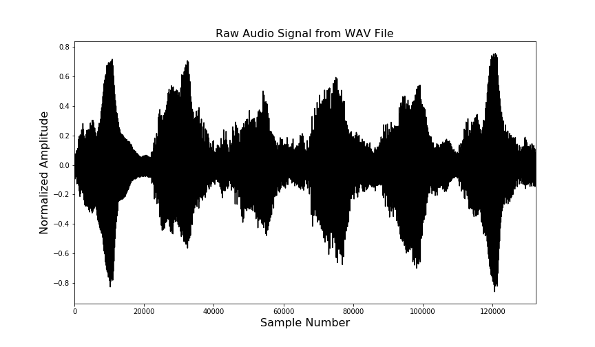
WAV files are the most common form of continuous representation because they contain an uncompressed, raw audio signal. This differs from mp3 files, for example, which compress the size of the file by discarding information about the audio signal.

The code block below shows how we can extract the sample rate, rate, and raw audio signal, signal, from a WAV file that contains a piece of music composed by Mozart. The sample rate is the number of times the audio signal is sampled each second. In our case, this value is 44100.

from scipy.io import wavfile

# Define data directory
data_dir = '../audio/'

# Extract sample rate and signal
rate, signal = wavfile.read(data_dir+'mozart.wav')

# Bound signal between -1 and 1
normalized_signal = signal / abs(max(signal))

The raw audio signal, signal, is an S x C tensor, where S is the number of samples and C is the number of channels. For simplicity, we will consider the case where C = 1. The plot below shows a three second interval of signal.

In general, using raw audio signals to train a model is considerably more challenging than using a discrete representation. A recent survey of deep learning methods for music generation examined 32 different methods of music generation in the literature. Among those, only three used continuous representations:

1. Audio Style Transfer
2. DeepAuto-Controller
3. WaveNet

Key Transposition

One method that can be used for either dimensionality reduction or data augmentation purposes is key transposition. This entails shifting each note's pitch by a fixed interval. If, for instance, a song contains a sequence where the pitch C₃ is followed by the pitch D₃ and we use a transposition that shifts all elements up by two pitches, then C₃ will become D₃ and D₃ will become E₃. For models that make use of key transposition, see Lim, Rhyu, and Lee (2018) and Sturm et al. (2016).

If we use key transposition for the purpose of dimensionality reduction, our goal will be to shift notes and chords such that we minimize the total number of unique notes and chords in our dataset. Since music tends to be written around certain groups of pitches called keys that sound good when played together, we can conveniently shift each song in our dataset into the same key.

This time, we'll import three submodules from music21:

1. converter, which we'll use to load a MIDI file and convert it into a stream object.
2. pitch, which we'll use to create our target pitch.
3. interval, which we'll use to compute the distance between our original key and our targeted key.

from music21 import converter, pitch, interval

# Define data directory
data_dir = '../audio/'

# Parse MIDI file
score = converter.parse(data_dir+'giuliani.mid')

# Identify and print original key
key = score.analyze('key')
print(key)
C major

# Compute interval between original key and target key
keyInterval = interval.Interval(key.tonic, pitch.Pitch('F'))

# Transpose song into F major
newScore = score.transpose(keyInterval)

# Print new key
print(newScore.analyze('key'))
F major

We first apply the .analyze('key') method to score, which identifies the stream object's key, which is C major. We then compute the interval between C major and our target key, F major. Notice that we access the pitch of the key object using .tonic. Furthermore, we create the targeted pitch using pitch.Pitch('F'). We then assign the output to keyInterval, which tells us the distance between our original and targeted keys.

Finally, we transpose the key using the .transpose() method and passing the interval, keyInterval. Printing the new key confirms that it is F major.

Octave Transposition

If we want to go further than key transposition, we can also transpose the octave to be higher or lower. Rather than transposing C major to F major, for instance, we can transpose C major to C major in a lower or higher octave. If we target the same set of octaves for each song, we will force all of our notes and chords to cluster together, reducing the dimensionality of the problem and making the model training process simpler. In the code block above, we could achieve this by specifying the octave of the pitch. For instance, instead of specifying pitch.Pitch('F') to compute the interval, we might use pitch.Pitch('F3').

Key and Octave Invariance

A natural alternative to dimensionality reduction is data augmentation. That is, rather than reducing the set of possible inputs and outputs, we expand the dataset by making changes to the existing data. We can also do this using key and octave transposition. However, instead of transposing all songs into a common key and clustering their notes in adjacent octaves, we would instead transpose all songs to all keys and all octaves. This would allow us to achieve key and octave invariance in the model we develop. See Briot, Hadjerest, and Pachet (2019) for a discussion of the use of transposition for the two different purposes.

Data Collection

We'll collect the MIDI files to train our model from Project Mutopia. Before we do any scraping, we'll first check the robots file, which is located at https://www.mutopiaproject.org/robots.txt, to make sure that we respect all requests for how automated interactions with the website should be handled. At the time this tutorial was written, the robots file contained the text in the code block below. User-agent: * indicates that the rule that follows applies to all users interacting with the website. Disallow:, followed by nothing, means that no restrictions are placed on scraping.

# Allow crawling of all content
User-agent: *
Disallow:

We will first import urlopen and urlretrieve from urllib.request, which we'll use to send get requests for each of the pages in the guitar section and then download each MIDI file linked to on the page. We'll import BeautifulSoup to parse the HTML returned by urlopen, allowing us to identify MIDI file links. Finally, we'll use the time module to pause for 10 seconds between downloads to avoid putting a strain on the website's resources.

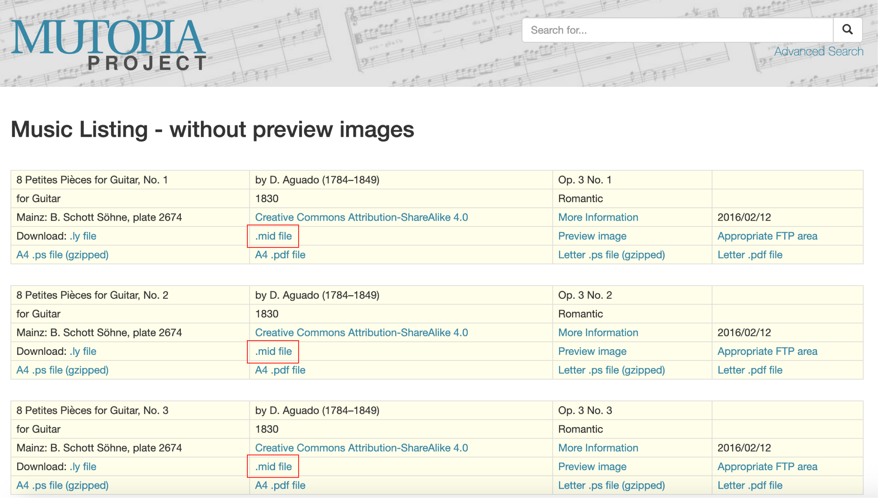
Each step of the main loop will check if the number of links on the page linkCount exceeds 0. If it does, it will construct the URL for the next page to navigate to, url, using the strings url0, url1, and the song number, songNumber. It will then open the url, parse the HTML, find all links on the page, reset linkCount to 0, and then step through each link in the list. If a link contains the substring .mid, then it points to a MIDI file and is downloaded using urlretrieve() to the directory specified by save_dir. Finally, we increment songNumber by 10, since each page contains 10 songs. We repeat this process until we encounter a page which contains fewer than 10 links.

!pip install bs4
from urllib.request import urlopen, urlretrieve
from bs4 import BeautifulSoup
import time

# Define save directory.
save_dir = '../guitar/'

# Define URL components
url0 = 'https://www.mutopiaproject.org/cgibin/make-table.cgi?startat='
url1 = '&searchingfor=&Composer=&Instrument=Guitar&Style=&collection=&id=&solo=&recent=&timelength=&timeunit=&lilyversion=&preview='

# Set initial values
songNumber = 0
linkCount = 10

# Locate and download each MIDI file
while linkCount > 0:
    url = url0 + str(songNumber) + url1
    html = urlopen(url)
    soup = BeautifulSoup(html.read())
    links = soup.find_all('a')
    linkCount = 0
    for link in links:
        href = link['href']
        if href.find('.mid') >= 0:
            linkCount = linkCount + 1
            urlretrieve(href, save_dir+href)
    songNumber += 10
    time.sleep(10.0)

For those interested in learning more about scraping, see DataCamp's Web Scraping with Python course and Web Scraping using Python tutorial.