Course
Use cutting-edge techniques with R, NLP and Machine Learning to model topics in text and build your own music recommendation system!
This is part Two-B of a three-part tutorial series in which you will continue to use R to perform a variety of analytic tasks on a case study of musical lyrics by the legendary artist Prince, as well as other artists and authors. The three tutorials cover the following:
- Part One: Lyric Analysis with NLP & Machine Learning with R
- Part Two-A: Tidy Sentiment Analysis in R
- Part Two-B: Machine Learning and NLP using R - Topic Modeling and Music Classification
- Part Three: Lyric Analysis: Predictive Analytics using Machine Learning with R
Imagine you are a Data Scientist working for NASA. You are asked to monitor two spacecraft intended for lunar orbits, which will study the moon's interactions with the sun. As with any spacecraft, there can be problems that are captured during test or post-launch. These anomalies are documented in natural language into nearly 20,000 problem reports. Your job is to identify the most popular topics and trending themes in the corpus of reports and provide prescriptive analysis results to the engineers and program directors, thus impacting the future of space exploration.
This is an example of a real-life scenario and should give you an idea of the power you'll have at your fingertips after learning how to use cutting-edge techniques, such as topic modeling with machine learning, Natural Language Processing (NLP) and R programming. Luckily, you don't have to work for NASA to do something just as innovative. In this tutorial, your mission, should you choose to accept it, is to learn about topic modeling and how to build a simple recommendation (a.k.a recommender) system based on musical lyrics and nonfiction books.
Just for Fun!
This has nothing to do with topic modeling, but just for fun, use a great package called circlize, introduced in a previous tutorial, to fire up those photoreceptors and enjoy this circle diagram of all the sources you'll use in this tutorial.
 library(jpeg)
library(circlize) #you'll use this package later
#read in the list of jpg files of album/book covers
files = list.files("jpg\\", full.names = TRUE)
#clean up the file names so we can use them in the diagram
removeSpecialChars <- function(x) gsub("[^a-zA-Z]", " ", x)
names <- lapply(files, removeSpecialChars)
names <- gsub("jpg","", names )

#read up on the circlize package for details
#but there will be comments in later sections
circos.clear()
circos.par("points.overflow.warning" = FALSE)
circos.initialize(names, xlim = c(0, 2))
circos.track(ylim = c(0, 1), panel.fun = function(x, y) {
  image = as.raster(readJPEG(files[CELL_META$sector.numeric.index]))
  circos.text(CELL_META$xcenter, CELL_META$cell.ylim[1] - uy(1.5, "mm"),
              CELL_META$sector.index,
              CELL_META$sector.index, facing = "clockwise", niceFacing = TRUE,
              adj = c(1, 0.5), cex = 0.9)
  circos.raster(image, CELL_META$xcenter, CELL_META$ycenter, width = "1.5cm",
        facing = "downward")
}, bg.border = 1, track.height = .4)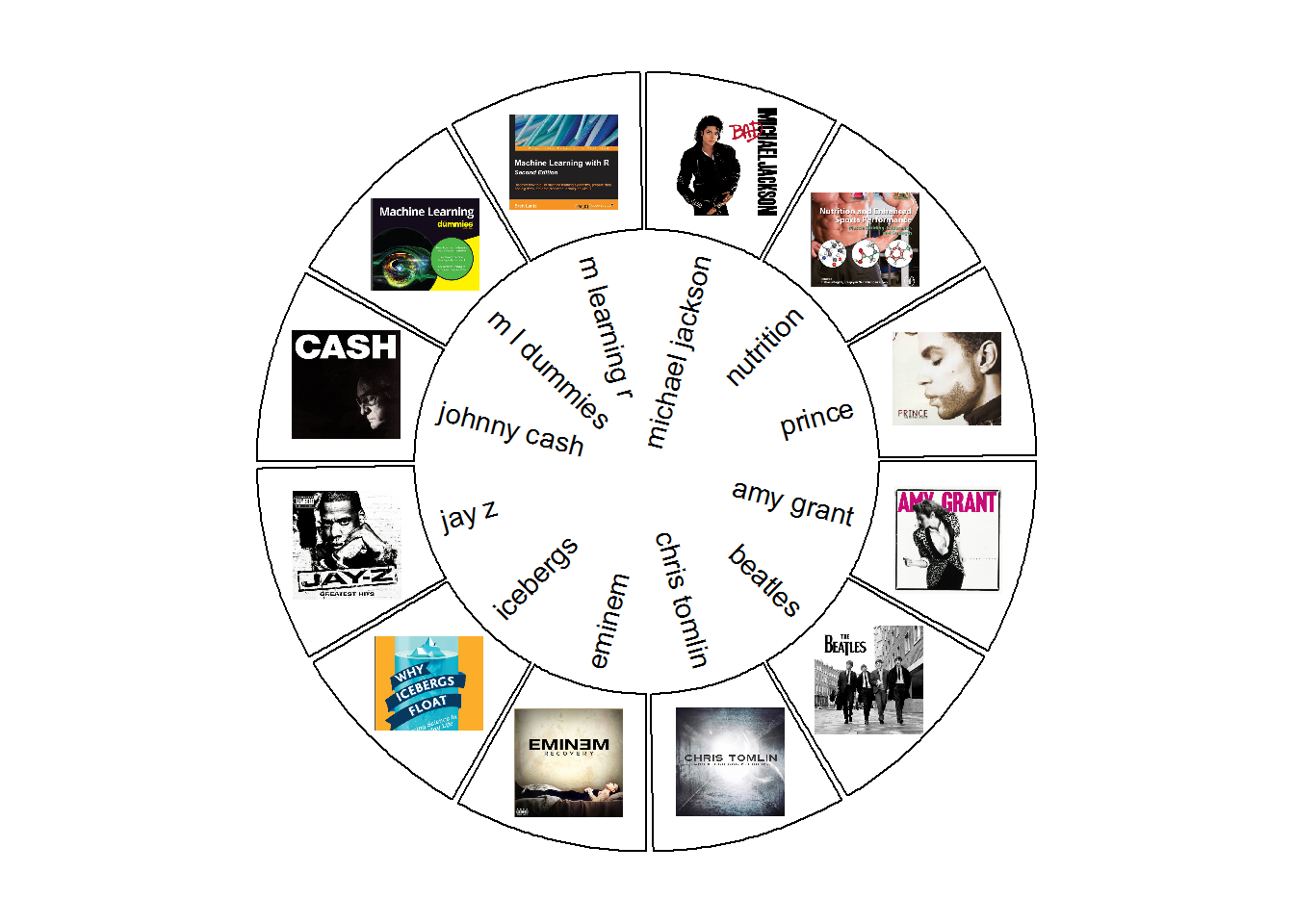
Structure
In previous tutorials, you studied the content of Prince's lyrics using word frequency, the tf-idf statistic, and sentiment analysis. You can get deeper insight into lyrics and other text by using the concept of topic modeling.
In this tutorial, you will build four models using Latent Dirichlet Allocation (LDA) and K-Means clustering machine learning algorithms. I will explain the algorithms later in the tutorial.
Model One utilizes text from Prince's lyrics combined with two nonfiction books. The objective of this model is to give you a simple example of using LDA, an unsupervised algorithm, to generate collections of words that together suggest themes. These themes are unlabeled and require human interpretation. Once you have identified a predefined number of themes, you will then take the results of your model and classify each song or book page into each category. A song may contain all the topics you've generated but may fit more cleanly into one over another. This is referred to as document classification, but since you know the writer of the document, you are essentially classifying writers into thematic groupings.
Model Two uses the Model One dataset and gives a quick glance into generating themes using a different algorithm, k-means, and how it may not be the best choice for topic modeling.
Once again using LDA, Model Three utilizes a larger dataset with multiple artists from different genres and more book authors. When you classify the majority of documents from an author/artist into their most likely topic, you have created the ability to group writers with similar thematic compositions. With a solid model, you should see similar genres appear in the same topic grouping. For example, rap artists would appear in one topic, and two books on a similar subject should appear together in a different topic. Thus, you could potentially recommend similar writers! Obviously, the writers and their genre are labeled, but the topics are not, and are therefore unsupervised.
Model Four uses LDA only on Prince's lyrics. This time you'll use an annotated dataset generated outside of this tutorial that has each word tagged as a part of speech (i.e. noun, verb, etc.) as well as the root form (lemmatized) of the word. You will also examine how a topic changes over time.
Introduction
NLP and Machine Learning are subfields of Artificial Intelligence. There have been recent attempts to use AI for songwriting. That's not the goal of this tutorial, but it's an example of how AI can be used as art. After all, the first three letters are A-R-T! Just for a moment, compare AI to songwriting: you can easily follow a pattern and create a structure (verse, chorus, verse, etc.), but what makes a song great is when the writer injects creativity into the process. In this tutorial, you'll need to exercise your technical skills to build models, but you'll also need to invoke your artistic creativity and develop the ability to interpret and explain your results.
Consider this: If topic modeling is an art, then lyrics are the code, songwriting is the algo-rhythm, and the song is the model! What's your analogy?
Typical recommendation systems are not based entirely on text. For example, Netflix can recommend movies based on previous choices and associated metadata. Pandora has a different approach and relies on a Music Genome consisting of 400 musical attributes, including melody, rhythm, composition and lyric summaries; however, this genome development began in the year 2000 and took five years and 30 experts in music theory to complete. There are plenty of research papers addressing movie recommendations based on plot summaries. Examples of music recommendation systems based on actual lyrical content are harder to find. Want to give it a try?
Prerequisites
Part Two-B of this tutorial series requires a basic understanding of tidy data - specifically packages such as dplyr and ggplot2. Practice with text mining using tidytext is also recommended, as it was covered in the previous tutorials. You'll also need to be familiar with R functions, as you will utilize a few to reuse your code for each model. In order to focus on capturing insights, I have included code that is designed to be used on your own dataset, but detailed explanation may require further investigation on your part.
Prepare your Questions
What can you do with topic modeling? Maybe there are documents that contain critical information to your business that you could mine. Maybe you could scrape data from Twitter and find out what people are saying about your company's products. Maybe you could build your own classification system to send certain documents to the right departments for analysis. There is a world of possibilities that you can explore! Go for it!
Why is Topic Modeling Useful?
Here are several applications of topic modeling:
- Document summaries: Use topic models to understand and summarize scientific articles enabling faster research and development. The same applies to historical documents, newspapers, blogs, and even fiction.
- Text classification: Topic modeling can improve classification by grouping similar words together in topics rather than using each word as an individual feature.
- Recommendation Systems: Using probabilities based on similarity, you can build recommendation systems. You could recommend articles for readers with a topic structure similar to articles they have already read.
- Do you have other ideas?
Prep Work
Libraries and Functions
The only new packages in this tutorial that are not in Part One or Part Two-A are topicmodels, tm, and plotly. You'll use the LDA() function from topicmodels which allows models to learn to distinguish between different documents. The tm package is for text mining, and you just use the inspect() function once to see the inside of a document-term matrix, which I'll explain later. You'll only use plotly once to create an interactive version of a ggplot2 graph.
 library(tidytext) #text mining, unnesting
library(topicmodels) #the LDA algorithm
library(tidyr) #gather()
library(dplyr) #awesome tools
library(ggplot2) #visualization
library(kableExtra) #create attractive tables
library(knitr) #simple table generator
library(ggrepel) #text and label geoms for ggplot2
library(gridExtra)
library(formattable) #color tile and color bar in `kables`
library(tm) #text mining
library(circlize) #already loaded, but just being comprehensive
library(plotly) #interactive ggplot graphs
The following functions were defined in previous tutorials with the exception of word_chart(); however, the content and description of word_chart() can also be found in Part Two-B. Primarily, you need to know that it uses ggplot() in a unique way to create a visual based on words rather than points.
 #define some colors to use throughout
my_colors <- c("#E69F00", "#56B4E9", "#009E73", "#CC79A7", "#D55E00", "#D65E00")

#customize ggplot2's default theme settings
#this tutorial doesn't actually pass any parameters, but you may use it again in future tutorials so it's nice to have the options
theme_lyrics <- function(aticks = element_blank(),
                         pgminor = element_blank(),
                         lt = element_blank(),
                         lp = "none")
{
  theme(plot.title = element_text(hjust = 0.5), #center the title
        axis.ticks = aticks, #set axis ticks to on or off
        panel.grid.minor = pgminor, #turn on or off the minor grid lines
        legend.title = lt, #turn on or off the legend title
        legend.position = lp) #turn on or off the legend
}

#customize the text tables for consistency using HTML formatting
my_kable_styling <- function(dat, caption) {
  kable(dat, "html", escape = FALSE, caption = caption) %>%
  kable_styling(bootstrap_options = c("striped", "condensed", "bordered"),
                full_width = FALSE)
}

word_chart <- function(data, input, title) {
  data %>%
  #set y = 1 to just plot one variable and use word as the label
  ggplot(aes(as.factor(row), 1, label = input, fill = factor(topic) )) +
  #you want the words, not the points
  geom_point(color = "transparent") +
  #make sure the labels don't overlap
  geom_label_repel(nudge_x = .2,
                   direction = "y",
                   box.padding = 0.1,
                   segment.color = "transparent",
                   size = 3) +
  facet_grid(~topic) +
  theme_lyrics() +
  theme(axis.text.y = element_blank(), axis.text.x = element_blank(),
        #axis.title.x = element_text(size = 9),
        panel.grid = element_blank(), panel.background = element_blank(),
        panel.border = element_rect("lightgray", fill = NA),
        strip.text.x = element_text(size = 9)) +
  labs(x = NULL, y = NULL, title = title) +
    #xlab(NULL) + ylab(NULL) +
  #ggtitle(title) +
  coord_flip()
}
Music and Books
In order to really see the power of topic modeling and classification, you'll not only use Prince's lyrics as with prior tutorials, but you'll also be working with several other artists from different genres recognized on the Billboard Charts. In addition, I've added a few books about different topics, such as sports nutrition, icebergs, and even machine learning! By having a varied dataset, you can classify documents into associated topics and distinguish between similar artists/authors.
Tip: I will refer to songs and the pages of books as documents, and musicians/authors as writers. In the code, you will see reference to the word source. This simply refers to which writer the data references. I'll use the word genre to refer to both the musical genre and the category of a book. Instead of using book author names, I used book titles, for clarity. These references will make sense as you progress through the tutorial.
Get the Data
In order to focus on modeling, I performed data conditioning outside of this tutorial and have provided you with all the data you need in these three files below with the following conditioning already applied:
- scraped the web for lyrics of eight artists
- used the
pdf_text()function from thepdftoolspackage to collect the content of four books (each page represents a distinct document) - cleaned all the data, removed stop words, and created the tidy versions using the
tidytextpackage described in Part One - combined and balanced the data such that each writer (source) has the same number of words
You will have three distinct datasets to work within this tutorial:
three_sources_tidy_balanced: contains Prince lyrics and two booksall_sources_tidy_balanced: contains lyrics from eight artists and four booksprince_tidy: contains only Prince lyrics
I've also included an annotated dataset of Prince's lyrics as well. I will explain what is meant by annotated when you get to Model Four.
 #Get Tidy Prince Dataset and Balanced Tidy Dataset of All Sources and 3 Sources

three_sources_tidy_balanced <- read.csv("three_sources_tidy_balanced.csv",
                                        stringsAsFactors = FALSE)

all_sources_tidy_balanced <- read.csv("all_sources_tidy_balanced.csv",
                                      stringsAsFactors = FALSE)

prince_tidy <- read.csv("prince_tidy.csv",
                        stringsAsFactors = FALSE)
Building Models with LDA
The main goal of topic modeling is finding significant thematically related terms (topics) in unstructured textual data measured as patterns of word co-occurrence. The basic components of topic models are documents, terms, and topics. Latent Dirichlet Allocation (LDA) is an unsupervised learning method which discovers different topics underlying a collection of documents, where each document is a collection of words. LDA makes the following assumptions:
- Every document is a combination of one or more topic(s)
- Every topic is a mixture of words
LDA seeks to find groups of related words. It is an iterative, generative algorithm. Here are the two main steps:
- During initialization, each word is assigned to a random topic
- The algorithm goes through each word iteratively and reassigns the word to a topic with the following considerations:
- the probability the word belongs to a topic
- the probability the document will be generated by a topic
The concept behind the LDA topic model is that words belonging to a topic appear together in documents. It tries to model each document as a mixture of topics and each topic as a mixture of words. (You may see this referred to as a mixed-membership model.) You can then use the probability that a document belongs to a particular topic to classify it accordingly. In your case, since you know the writer of the document from the original data, you can then recommend an artist/author based on similar topic structures. Now it's time to take a look at an example.
Model One: LDA for Three Writers
Examine the Data
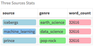
For this model, you will use the dataset with a combination of three distinct writers (i.e. sources) and look for hidden topics. In order to help you understand the power of topic modeling, these three chosen sources are very different and intuitively you know they cover three different topics. As a result, you'll tell your model to create three topics and see how smart it is. First you want to examine your dataset using your my_kable_styling() function along with color_bar() and color_tile() from the formattable package.
 #group the dataset by writer (source) and count the words
three_sources_tidy_balanced %>%
  group_by(source) %>%
  mutate(word_count = n()) %>%
  select(source, genre, word_count) %>% #only need these fields
  distinct() %>%
  ungroup() %>%
  #assign color bar for word_count that varies according to size
  #create static color for source and genre
  mutate(word_count = color_bar("lightpink")(word_count),
         source = color_tile("lightblue","lightblue")(source),
         genre = color_tile("lightgreen","lightgreen")(genre)) %>%
  my_kable_styling("Three Sources Stats")
Here you will use Prince lyrics, a book called "Machine Learning For Dummies", and another book called "Why Icebergs Float", each having over 30,000 (non-distinct) words.
Create the Document-Term Matrix
Since you currently have a balanced, tidy dataset with Prince lyrics and two books, you'll first want to create a document-term matrix (DTM) in which each document is a row, and each column is a term. This format is required for the LDA algorithm. A document refers to a song in the lyrics and a page number in the books. First, you'll take your tidy data and count the words in a document, then pipe that into tidytext's cast_dtm() function where document is the name of the field with the document name and word is the name of the field with the term. There are other parameters you could pass, but these two are required.
 three_sources_dtm_balanced <- three_sources_tidy_balanced %>%
  #get word count per document to pass to cast_dtm
  count(document, word, sort = TRUE) %>%
  ungroup() %>%
  #create a DTM with docs as rows and words as columns
  cast_dtm(document, word, n)
#examine the structure of the DTM
three_sources_dtm_balanced

<<DocumentTermMatrix (documents: 1449, terms: 13608)>>
Non-/sparse entries: 71386/19646606
Sparsity           : 100%
Maximal term length: 27
Weighting          : term frequency (tf)
This tells you how many documents and terms you have and that this is a very sparse matrix. The word sparse implies that the DTM contains mostly empty fields. Because of the vast vocabulary of possible terms from all documents, only a few will be used in each individual document.
If you look at the contents of a few rows and columns of the DTM using the inspect() function from the tm package, you'll see that each row is a document and each column is a term. (Feel free to use str() to see the actual structure.)
 #look at 4 documents and 8 words of the DTM
inspect(three_sources_dtm_balanced[1:4,1:8])
<<DocumentTermMatrix (documents: 4, terms: 8)>>
Non-/sparse entries: 9/23
Sparsity : 72%
Maximal term length: 9
Weighting : term frequency (tf)
Sample :
Terms
Docs beautiful dance party push rock roll shake style
party up 0 0 40 0 1 2 0 0
push it up 0 1 1 56 0 0 0 0
shake 0 0 1 0 0 0 52 0
style 0 0 0 0 0 0 0 32Set Variables
Now that you know what is needed as input to build your model, set two variables that you can simply reset when constructing each model. You'll call these source_dtm and source_tidy.
 #assign the source dataset to generic var names
#so we can use a generic function per model
source_dtm <- three_sources_dtm_balanced
source_tidy <- three_sources_tidy_balanced
Fit the Model
Finally, you get to the fun part of fitting the model. The code is simple, but to be a good Data Scientist, you'll want to understand what is happening behind the scenes. Although this is a cursory description, there is a wealth of information on LDA online. For your purposes, you'll just need to know four parameters: the input, the number of topics, the sampling method and the seed.
Since you know your dataset contains three distinct writers, you'll set k to 3 and set seed to a constant so that you can obtain repeatable results. There are other control parameters, thus the list format in the code, but you'll just use seed for now. The method parameter defines the sampling algorithm to use. You'll use the GIBBS sampling method. The default is VEM, but in my experience, it does not perform as well as the alternative GIBBS sampling method.
A short technical explanation of GIBBS sampling is that it performs a random walk that starts at some point which you can initialize (you'll just use the default of 0) and at each step moves plus or minus one with equal probability. Read a detailed description here if you are interested in the details.
Note: I have glossed over the details of the LDA algorithm. Although you don't need to understand the statistical theory in order to use it, I would suggest that you read this document by Ethen Liu which provides a solid explanation.
 k <- 3 #number of topics
seed = 1234 #necessary for reproducibility
#fit the model passing the parameters discussed above
#you could have more control parameters but will just use seed here
lda <- LDA(source_dtm, k = k, method = "GIBBS", control = list(seed = seed))
#examine the class of the LDA object
class(lda)
[1] "LDA_Gibbs"
attr(,"package")
[1] "topicmodels"You can see here that this created an LDA_Gibbs object with three topics. I didn't run str(lda) here because of the large output, but go ahead and do it on your own to see what it contains.
The next step is to open up that object and see what the results are. You can use the tidy() function to put it in a format that is easy to understand. Within the call to tidy() pass the LDA object and beta for the matrix argument. Passing beta provides you with the per-topic-per-word probabilities from the model. The following example, using the term iceberg, shows the probability of that word being in each topic. The word iceberg has a higher probability of being generated in Topic 1.
 #convert the LDA object into a tidy format
#passing "beta" shows the word probabilities
#filter on the word iceberg as an example
#results show probability of iceberg for each topic
tidy(lda, matrix = "beta") %>% filter(term == "iceberg")
[# A tibble: 3 x 3 topic term beta 1 1 iceberg 0.000198
2 2 iceberg 0.00000292 3 3 iceberg 0.00000315]
Identify Themes with Top Words
To understand the model clearly, you need to see what terms are in each topic. Build a function that will tidy the LDA model, and extract the top terms for each topic. In other words, the terms per topic with the largest beta values. Inside this function, you'll refer to word_chart() that you built earlier to generate a nice display of the three topics and the top words. Set num_words to 10 for this example, but you can play around with that number to get different perspectives on the topics.
 num_words <- 10 #number of words to visualize

#create function that accepts the lda model and num word to display
top_terms_per_topic <- function(lda_model, num_words) {

  #tidy LDA object to get word, topic, and probability (beta)
  topics_tidy <- tidy(lda_model, matrix = "beta")


  top_terms <- topics_tidy %>%
  group_by(topic) %>%
  arrange(topic, desc(beta)) %>%
  #get the top num_words PER topic
  slice(seq_len(num_words)) %>%
  arrange(topic, beta) %>%
  #row is required for the word_chart() function
  mutate(row = row_number()) %>%
  ungroup() %>%
  #add the word Topic to the topic labels
  mutate(topic = paste("Topic", topic, sep = " "))
  #create a title to pass to word_chart
  title <- paste("LDA Top Terms for", k, "Topics")
  #call the word_chart function you built in prep work
  word_chart(top_terms, top_terms$term, title)
}
#call the function you just built!
top_terms_per_topic(lda, num_words)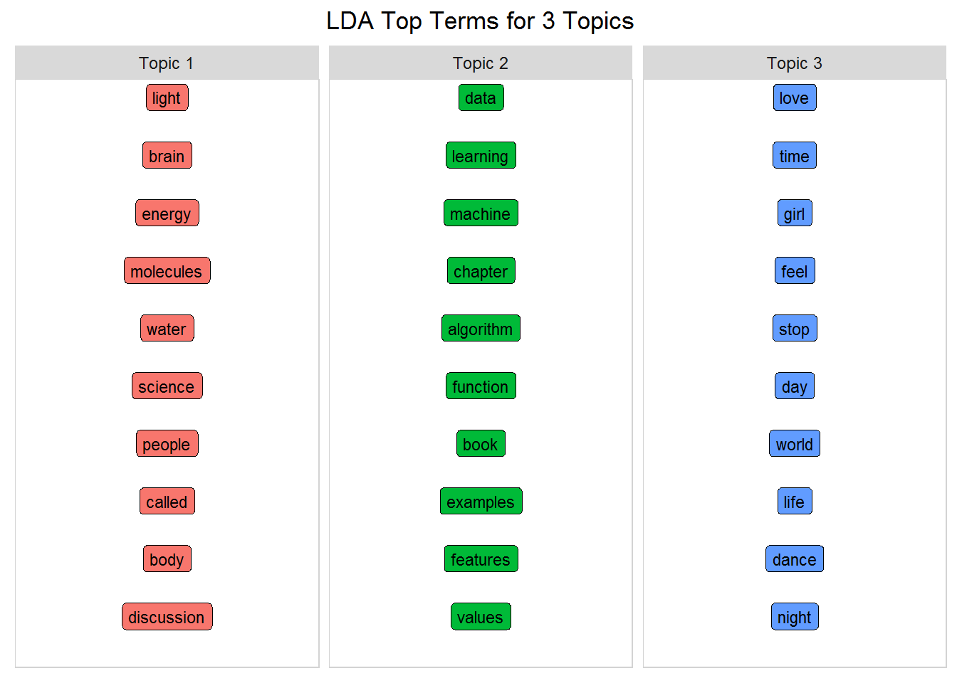
Unsupervised learning always requires human interpretation...but these topics clearly reflect the three sources of Icebergs, Machine Learning, and Prince! Even though this is a very simple example, it is pretty amazing when you think about the possibilities!
Classify Documents
In addition to estimating each topic as a mixture of words, LDA also shows each document as a mixture of topics. This time when you tidy the LDA model, use matrix = "gamma" and you'll get the per-document-per-topic probabilities. For example, look at Prince's song 1999. Here you see that, just as a word will be associated with multiple topics, the same is true for documents. This refers back to that mixed-membership concept. Below you can see that 1999 is most likely to appear in Topic 3.
 #this time use gamma to look at the prob a doc is in a topic
#just look at the Prince song 1999 as an example
tidy(lda, matrix = "gamma") %>% filter(document == "1999")
# A tibble: 3 x 3
document topic gamma
<chr> <int> <dbl>
1 1999 1 0.170
2 1999 2 0.170
3 1999 3 0.661This song belongs to each topic, but at a different percentage, represented by the gamma value. Some documents fit in some topics better than others. As shown above, 1999 has a higher gamma value for Topic 3.
Chord Diagram
In order to clarify your understanding of what LDA does, take a look at this circle plot. This plot shows what percentage of docs from each source belongs to each topic. In order to create it, join the tidy LDA model back to source_tidy where you stored the actual source (i.e. the writer), and join by document. Then if you do the proper grouping, you can get the average gamma value per source, per topic. Now you can see, for each source, into which topic the majority of documents fall.
Take a second to really examine it if you haven't used circle plots before. (Check out Part Two-A for practice with chordDiagrams() and the circlize package. All you'll ever need to know about the package is covered in this book by Zuguang Gu.)
 #using tidy with gamma gets document probabilities into topic
#but you only have document, topic and gamma
source_topic_relationship <- tidy(lda, matrix = "gamma") %>%
  #join to orig tidy data by doc to get the source field
  inner_join(three_sources_tidy_balanced, by = "document") %>%
  select(source, topic, gamma) %>%
  group_by(source, topic) %>%
  #get the avg doc gamma value per source/topic
  mutate(mean = mean(gamma)) %>%
  #remove the gamma value as you only need the mean
  select(-gamma) %>%
  #removing gamma created duplicates so remove them
  distinct()

#relabel topics to include the word Topic
source_topic_relationship$topic = paste("Topic", source_topic_relationship$topic, sep = " ")

circos.clear() #very important! Reset the circular layout parameters
#assign colors to the outside bars around the circle
grid.col = c("prince" = my_colors[1],
             "icebergs" = my_colors[2],
             "machine_learning" = my_colors[3],
             "Topic 1" = "grey", "Topic 2" = "grey", "Topic 3" = "grey")

# set the global parameters for the circular layout. Specifically the gap size (15)
#this also determines that topic goes on top half and source on bottom half
circos.par(gap.after = c(rep(5, length(unique(source_topic_relationship[[1]])) - 1), 15,
                         rep(5, length(unique(source_topic_relationship[[2]])) - 1), 15))
#main function that draws the diagram. transparancy goes from 0-1
chordDiagram(source_topic_relationship, grid.col = grid.col, transparency = .2)
title("Relationship Between Topic and Source")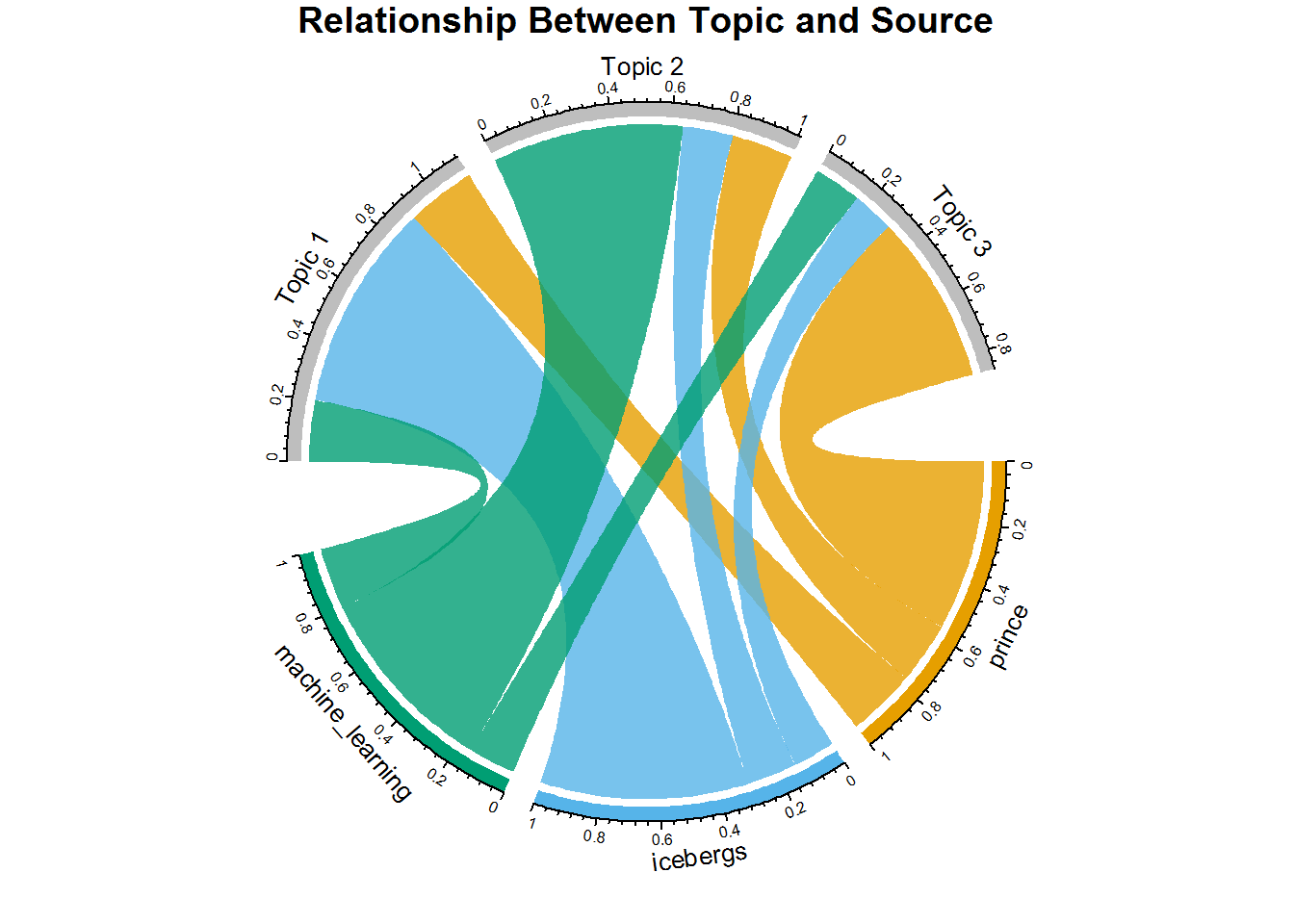
This is a really interesting way to see that even though the documents from each source appear in each topic, each source clearly has a majority in a specific topic. For example, Prince songs are mostly associated with Topic 3 as that chord is larger than the chords going to topics one and two. The same thing occurs for Icebergs and Topic 1, and Machine Learning and Topic 2. Once you see the pattern here, it becomes very clear what is happening.
If you think about what you've just done, you've actually classified documents into Topics based on the mean of gamma for a topic/source. If you know the writer of a document, and you know the writer composes most lyrics or books on a specific topic, you might assume that artists of similar genres would fall into the same topics and therefore you can recommend writers that are similar... When you look at the larger dataset, you'll put this exercise to practice.
Top Documents Per Topic
Now look at the individual document level and view the top documents per topic.
 number_of_documents = 5 #number of top docs to view
title <- paste("LDA Top Documents for", k, "Topics")

#create tidy form showing topic, document and its gamma value
topics_tidy <- tidy(lda, matrix = "gamma")

#same process as used with the top words
top_documents <- topics_tidy %>%
  group_by(topic) %>%
  arrange(topic, desc(gamma)) %>%
  slice(seq_len(number_of_documents)) %>%
  arrange(topic, gamma) %>%
  mutate(row = row_number()) %>%
  ungroup() %>%
  #re-label topics
  mutate(topic = paste("Topic", topic, sep = " "))

title <- paste("LDA Top Documents for", k, "Topics")
word_chart(top_documents, top_documents$document, title)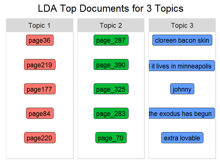
Identify Artists/Authors
Since you may not know the nomenclature of the document/song titles (i.e. pages with an underscore are from the machine learning book), I'll replace the document name with the source name.
 title <- paste("Sources for Top Documents for", k, "Topics")

topics_tidy <- tidy(lda, matrix = "gamma")

top_sources <- top_documents %>%
  #join back to the tidy form to get the source field
  inner_join(source_tidy) %>%
  select(document, source, topic) %>%
  distinct() %>%
  group_by(topic) %>%
  #needed by word_chart (not relevant here)
  mutate(row = row_number()) %>%
  ungroup()

word_chart(top_sources, top_sources$source, title)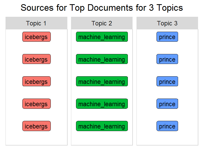
The top documents for each topic as shown in the previous chart are replaced by their source. Your code has done well at classifying these documents because they fell into the same category (at least for these top 5)! The big question is whether or not this works with more than just three sources. If your results are accurate, you can then recommend writers with similar topics.
Model Two: K-Means for Three Writers
You will create your second model using a different machine learning technique: the k-means algorithm. As with LDA, k-means is an unsupervised learning algorithm and requires you to decide the number of topics ahead of time. In contrast to the LDA mixed-membership model, k-means partitions the documents into apparent disjoint clusters (i.e. topics). Here, the algorithm clusters documents into different groups based on a similarity measure. It transforms documents to a numeric vector with weights assigned to words per document (similar to tf-idf). Each document will show up in exactly one cluster. This is called hard clustering. The output is a set of clusters along with their documents. In contrast, LDA is a fuzzy (soft) clustering technique where a data point can belong to more than one cluster.
So conceptually, when applied to natural language, LDA should give more realistic results than k-means for topic assignment, given that text usually entails more than one topic. Build your model now, examine the k-means object, and see if your assumption holds true.
Set Variables and Fit the Model
 #use the same three sources you started with
source_dtm <- three_sources_dtm_balanced
source_tidy <- three_sources_tidy_balanced

#Set a seed for replicable results
set.seed(1234)
k <- 3
kmeansResult <- kmeans(source_dtm, k)
str(kmeansResult)
List of 9
$ cluster : Named int [1:1449] 1 3 2 2 3 1 3 2 2 3 ...
..- attr(*, "names")= chr [1:1449] "push it up" "shake" "party up" "style" ...
$ centers : num [1:3, 1:13608] 42 0.01065 0.00758 0 0.01141 ...
..- attr(*, "dimnames")=List of 2
.. ..$ : chr [1:3] "1" "2" "3"
.. ..$ : chr [1:13608] "push" "shake" "party" "style" ...
$ totss : num 237535
$ withinss : num [1:3] 640 202211 28285
$ tot.withinss: num 231137
$ betweenss : num 6398
$ size : int [1:3] 2 1315 132
$ iter : int 3
$ ifault : int 0
- attr(*, "class")= chr "kmeans"The structure of the k-means object reveals two important pieces of information: clusters and centers. You can use the format below to see the contents of each variable for the song 1999 and the word party which appears in that song.
head(kmeansResult$cluster["1999"])1999
2head(kmeansResult$centers[,"party"])1 2 3
0.5000000 0.1269962 0.1439394These fields show that 1999 is placed in a single cluster (cluster two), and party is in all three clusters, but falls mainly in cluster one. So now look at the top words based on the centers values to identify themes.
Identify K-Means Themes with Top Words
Remember that this dataset contains three sources: Prince, Icebergs, and Machine Learning. Print the top words for each cluster and compare your results to the LDA output. You'll need to manipulate the format of the data just a bit in order to use your word_chart() function. You can follow along with the code, but the details are not as important here as the actual analysis of the top words.
 num_words <- 8 #number of words to display
#get the top words from the kmeans centers
kmeans_topics <- lapply(1:k, function(i) {
  s <- sort(kmeansResult$centers[i, ], decreasing = T)
  names(s)[1:num_words]
})

#make sure it's a data frame
kmeans_topics_df <- as.data.frame(kmeans_topics)
#label the topics with the word Topic
names(kmeans_topics_df) <- paste("Topic", seq(1:k), sep = " ")
#create a sequential row id to use with gather()
kmeans_topics_df <- cbind(id = rownames(kmeans_topics_df),
                          kmeans_topics_df)
#transpose it into the format required for word_chart()
kmeans_top_terms <- kmeans_topics_df %>% gather(id, 1:k)
colnames(kmeans_top_terms) = c("topic", "term")

kmeans_top_terms <- kmeans_top_terms %>%
  group_by(topic) %>%
  mutate(row = row_number()) %>% #needed by word_chart()
  ungroup()

title <- paste("K-Means Top Terms for", k, "Topics")
word_chart(kmeans_top_terms, kmeans_top_terms$term, title)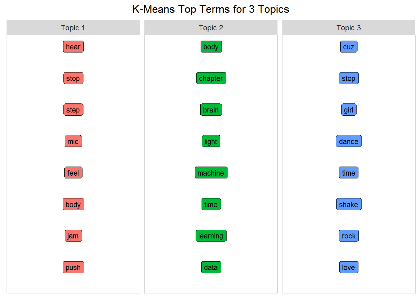
The k-means algorithm is smart enough to separate topics between books and music. In other words, Topics 1 and 3 are clearly Prince themes, and Topic 2 is a combination of the two books. However, it was not able to distinguish between the two books themselves as you were able to do using LDA. K-means can be tuned for better performance, but so can LDA. At a quick glance, with default parameters, k-means does not seem to perform as well as LDA, and in fact, hard clustering is typically not used as much for topic modeling. (For another option, check out the mallet package.)
Model Three: LDA for 12 Writers
For this model, you will use the LDA algorithm on the dataset with 12 different sources/writers covering multiple genres. The dataset is already balanced with a similar number of documents and words per writer. Here is an overview of the data:
Examine the Data
 all_sources_tidy_balanced %>%
  group_by(source) %>%
  #get the word count and doc count per source
  mutate(word_count = n(),
         source_document_count = n_distinct(document)) %>%
  select(source, genre, word_count, source_document_count) %>%
  distinct() %>%
  ungroup() %>%
  #bars change size according to number
  #tiles are static sizes
  mutate(word_count = color_bar("lightpink")(word_count),
         source_document_count = color_bar("lightpink")(source_document_count),
         source = color_tile("lightblue","lightblue")(source),
         genre = color_tile("lightgreen","lightgreen")(genre)) %>%
  my_kable_styling("All Sources Stats")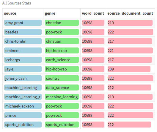
This dataset contains a wide variety of artists ranging from Prince, to Johnny Cash (country), to Eminem (rap) as well as four distinct books. These artists were chosen because they were ranked as most prolific in their respective genres. The content was scraped off a lyrics website. Although there are two machine learning books, one is focused on general data science and one is more about machine learning specific to R programming. All books are available as downloadable PDFs. (The raw PDFs are not needed for this analysis as the tidy versions were provided).
Just a quick housecleaning step: some of the genre descriptions are too long for our charts, so create abbreviated forms to make them more readable.
 all_sources_tidy_balanced <- all_sources_tidy_balanced %>%
  mutate(source = ifelse(source == "machine_learning", "m_learn",
         ifelse(source == "machine_learning_r", "m_learn_r",
         ifelse(source == "michael_jackson", "mi_jackson",
         ifelse(source == "sports_nutrition", "nutrition", source))))) %>%
  mutate(genre = ifelse(genre == "machine_learning", "m_learn",
                 ifelse(genre == "sports_nutrition", "nutrition", genre)))
Create the DTM and set the variables
 #this time use the dataset with 12 sources
all_sources_dtm_balanced <- all_sources_tidy_balanced %>%
  count(document, word, sort = TRUE) %>%
  ungroup() %>%
  cast_dtm(document, word, n)

source_dtm <- all_sources_dtm_balanced
source_tidy <- all_sources_tidy_balanced
Fit the Model and Identify Themes
This time you have twelve writers and eight genres. I'm hoping that writers from the same genre will get grouped into the same topic. That's the real test. So, set the number of topics to eight and fit the model again using this larger dataset.
 k <- 8 #number of topics chosen to match the number of genres
num_words <- 10 #number of words we want to see in each topic
seed = 1234 #make it repeatable
#same as before
lda <- LDA(source_dtm, k = k, method = "GIBBS", control = list(seed = seed))

top_terms_per_topic(lda, num_words)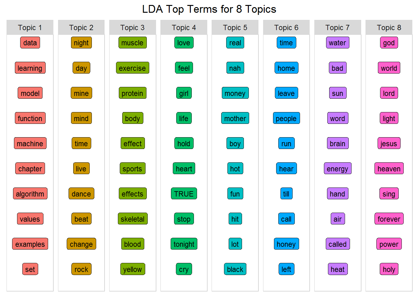
Not to influence your opinion, but my reaction is: "Wow"! Given the input for this model, can you see the themes? Look at each topic and try to match them to the eight known genres. Some will be hard to distinguish, but others will be fairly obvious. For example, here are some possibilities for interpretation:
- Topic One - machine learning and data science
- Topic Two - pop/rock
- Topic Three - sports nutrition
- Topic Four - country
- Topic Five - hip-hop-rap
- Topic Six - country or pop-rock
- Topic Seven - icebergs, earth science
- Topic Eight - religious
Don't forget about the mixed-membership concept and that these topics are not meant to be completely disjoint, but I was amazed to see the results as discrete as you see here. Just as a side note: the LDA algorithm takes more parameters than you used and thus you can tune your model to be even stronger.
This next part is really exciting. How can you make it easier to see what these topics are about? In most cases, it's tough to interpret, but with the right dataset, your model can perform well. If your model can determine which documents are more likely to fall into each topic, you can begin to group writers together. And since in your case you know the genre of a writer, you can validate your results - to a certain extent! The first step is to classify each document.
Classify Documents
Chord Diagram
As a reminder, each document contains multiple topics, but at different percentages represented by the gamma value. Some documents fit some topics better than others. This plot shows the average gamma value of documents from each source for each topic. This is the same approach you used above with three writers, except this time you'll look at the genre field. It is a fantastic way of showing the relationship between the genre of the writers and the topics.
 source_topic_relationship <- tidy(lda, matrix = "gamma") %>%
  #join to the tidy form to get the genre field
  inner_join(source_tidy, by = "document") %>%
  select(genre, topic, gamma) %>%
  group_by(genre, topic) %>%
  #avg gamma (document) probability per genre/topic
  mutate(mean = mean(gamma)) %>%
  select(genre, topic, mean) %>%
  ungroup() %>%
  #re-label topics
  mutate(topic = paste("Topic", topic, sep = " ")) %>%
  distinct()

circos.clear() #very important! Reset the circular layout parameters
#this is the long form of grid.col just to show you what I'm doing
#you can also assign the genre names individual colors as well
grid.col = c("Topic 1" = "grey", "Topic 2" = "grey", "Topic 3" = "grey",
             "Topic 4" = "grey", "Topic 5" = "grey", "Topic 6" = "grey",
             "Topic 7" = "grey", "Topic 8" = "grey")

#set the gap size between top and bottom halves set gap size to 15
circos.par(gap.after = c(rep(5, length(unique(source_topic_relationship[[1]])) - 1), 15,
                         rep(5, length(unique(source_topic_relationship[[2]])) - 1), 15))
chordDiagram(source_topic_relationship,  grid.col = grid.col, annotationTrack = "grid",
             preAllocateTracks = list(track.height = max(strwidth(unlist(dimnames(source_topic_relationship))))))
#go back to the first track and customize sector labels
#use niceFacing to pivot the label names to be perpendicular
circos.track(track.index = 1, panel.fun = function(x, y) {
  circos.text(CELL_META$xcenter, CELL_META$ylim[1], CELL_META$sector.index,
              facing = "clockwise", niceFacing = TRUE, adj = c(0, 0.5))
}, bg.border = NA) # here set bg.border to NA is important
title("Relationship Between Topic and Genre")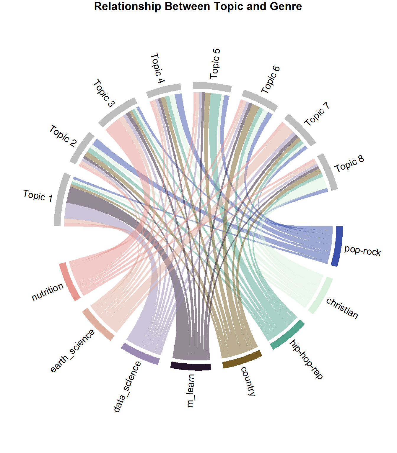
Every chord (i.e link) represents the mean gamma value of documents per genre that belong to a topic. If you look at the sports_nutrition section, you can see that the chord to Topic 3 is larger than its other chords. This means that more sports nutrition pages fall into that topic. Clearly, the majority of Machine Learning and Data Science pages fall into Topic 1; the majority of Earth Science documents fall into Topic 7, and as you may expect, Pop-Rock is pretty well divided among multiple topics. This makes perfect sense because, by definition, Pop stands for popular and is a generalized genre. Rap-Hip-Hop, on the other hand, is more common in Topic 5. So what can you do with this information? You can make recommendations to listeners based on thematic content!
Of course, lyrical content need not be the only feature used by recommendation systems but could be combined with metadata such as rhythm, instrumentation, tempo, etc.., for a better listening experience.
Recommend Similar Writers
Now that you can see the relationship between documents and topics, group by source (i.e. writer) and topic and get the sum of gamma values per group. Then select the writer with the highest topic_sum for each topic using top_n(1). Since you'll want to do the same thing for genre as you're doing here with writer, create a function called top_items_per_topic() and pass source as the type. This way you'll be able to call it again when you classify documents by genre.
This is the critical moment where you actually map the writer to a specific topic. What do you expect will happen?
 #this function can be used to show genre and source via passing the "type"
top_items_per_topic <- function(lda_model, source_tidy, type) {
  #get the tidy version by passing gamma for the per document per topic probs
  document_lda_gamma <- tidy(lda_model, matrix = "gamma") %>%
  #join to the tidy form to get source and genre
  inner_join(source_tidy) %>%
  select(document, gamma, source, genre, topic) %>%
  distinct() %>% #remove duplicates
  #group so that you can get sum per topic/source
  group_by(source, topic) %>%
  #sort by decending gamma value
  arrange(desc(gamma)) %>%
  #create the sum of all document gamma vals per topic/source. Important!
  mutate(topic_sum = sum(gamma)) %>%
  select(topic, topic_sum, source, genre) %>%
  distinct() %>%
  ungroup() %>%
  #type will be either source or genre
  group_by(source, genre ) %>%
  #get the highest topic_sum per type
  top_n(1, topic_sum) %>%
  mutate(row = row_number()) %>%
  mutate(label = ifelse(type == "source", source, genre),
         title = ifelse(type == "source", "Recommended Writers Per Topic",
                        "Genres Per Topic")) %>%
  ungroup() %>%
   #re-label topics
  mutate(topic = paste("Topic", topic, sep = " ")) %>%
  select(label, topic, title)

#slightly different format from word_chart input, so use this version
document_lda_gamma %>%
#use 1, 1, and label to use words without numeric values
ggplot(aes(1, 1, label = label, fill = factor(topic) )) +
  #you want the words, not the points
  geom_point(color = "transparent") +
  #make sure the labels don't overlap
  geom_label_repel(nudge_x = .2,
                   direction = "y",
                   box.padding = 0.1,
                   segment.color = "transparent",
                   size = 3) +
  facet_grid(~topic) +
  theme_lyrics() +
  theme(axis.text.y = element_blank(), axis.text.x = element_blank(),
        axis.title.y = element_text(size = 4),
        panel.grid = element_blank(), panel.background = element_blank(),
        panel.border = element_rect("lightgray", fill = NA),
        strip.text.x = element_text(size = 9)) +
  xlab(NULL) + ylab(NULL) +
  ggtitle(document_lda_gamma$title) +
  coord_flip()
}

top_items_per_topic(lda, source_tidy, "source")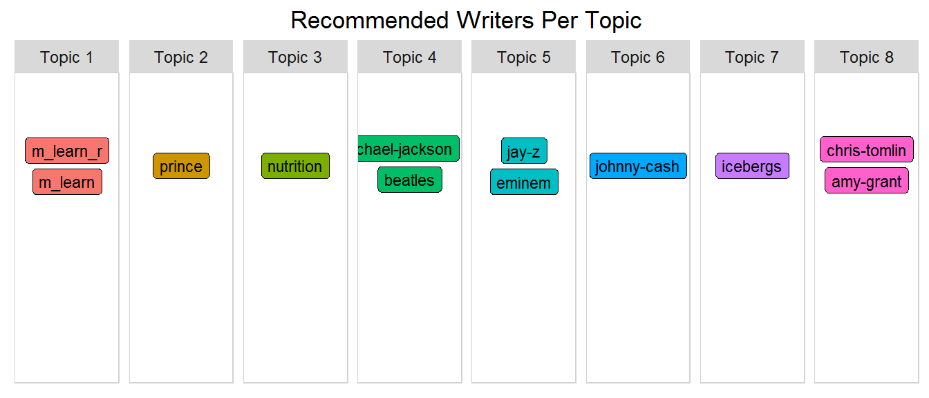
This is exciting! However, since you may not know these artists very well, I'll make things clear by replacing the writer with the genre. Get ready...
Recommend Similar Documents by Genre
top_items_per_topic(lda, source_tidy, "genre")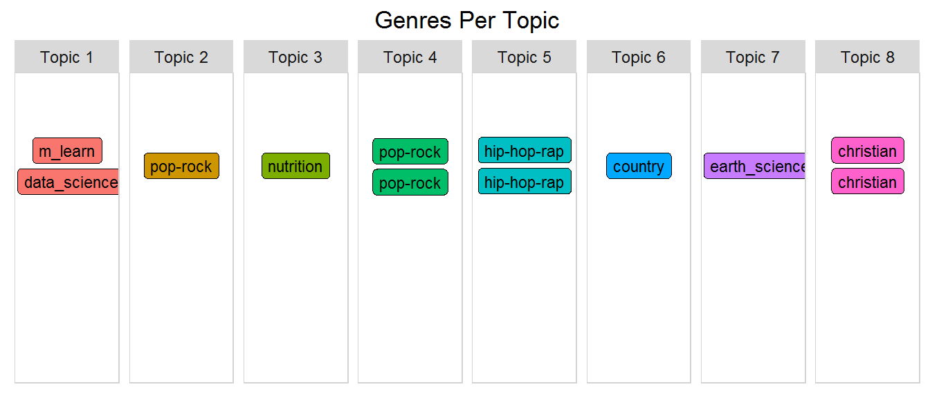
The hip-hop-rap artists are grouped together; the Christian artists are together; two of the pop-rock artists are together, and each book has its own topic! It's pretty amazing to see that unsupervised learning can produce results like this (recognizing different genres) based entirely on text. What would happen if you chose a different number of topics? What genres would it combine or separate? Maybe you could give it a try on your own. For now, your next model will focus on the Prince dataset you used in the previous tutorials.
Model Four: LDA for Prince Songs
For this model, you will use your dataset with only Prince songs. Although there are distinct topics covered in lyrics, it is often the case that a single song covers more than one topic. When your dataset only has one artist, your topics are going to be more mixed and less disjoint. This makes interpretation a very critical step. Instead of using the raw data from Prince's lyrics, you will use a slightly modified version as described below.
Use NLP to Improve Model
Previously you have used words as they appear in the text. But now you'll use an annotated form of the data resulting from a powerful NLP package called cleanNLP. This package is a tidy data model for Natural Language Processing that provides annotation tasks such as tokenization, part of speech tagging, named entity recognition, entity linking, sentiment analysis, and many others. This exercise was performed outside of this tutorial, but I have provided all you'll need for topic modeling.
Examine NLP Output
In the annotated dataset, there is one row for every word in the corpus of Prince's lyrics with important information about each word.
Take a closer look at the tokenized annotation object by examining the field names.
 #read in the provided annotated dataset
prince_annotated <- read.csv("prince_data_annotated.csv")
#look at the fields provided in the dataset
names(prince_annotated)
[1] "X" "id" "sid" "tid" "word"
[6] "lemma" "upos" "pos" "cid" "pid"
[11] "case" "definite" "degree" "foreign" "gender"
[16] "mood" "num_type" "number" "person" "poss"
[21] "pron_type" "reflex" "tense" "verb_form" "voice"For now, you will only utilize two pieces of information:
- lemma: the lemmatized word form (i.e. the reduced version of an inflected word to its base form)
- upos: the universal part of speech of each word
The word field is the original word and lemma is the lemmatized version. upos is the universal part of speech code. If you call table() on upos you will see the count of words that fall into each tagged part of speech. (Note that some words may be tagged multiple times)
table(prince_annotated$upos)ADJ ADP ADV AUX CCONJ DET INTJ NOUN NUM PART PRON PROPN
15193 19157 20439 19855 5601 20777 5399 48047 5439 10087 50932 523
SCONJ SYM VERB X
5626 72 43673 3095To give you an idea of what the data looks like, zoom in on a couple of songs where the lemma is not the same as the original word, and remove the stop words.
 prince_annotated %>%
  #most lemmas are the same as the raw word so ignore those
  filter((as.character(word) != as.character(lemma))
         & (id %in% c("broken", "1999"))) %>% #filter on 2 songs
  anti_join(stop_words) %>%
  select(song = id, word, lemma, upos) %>%
  distinct() %>%
  my_kable_styling("Annotated Subset")
This shows how you can be very selective in what you choose to put into your models (i.e. the word, the lemma, or a certain part of speech). It's really a judgment call about whether to use the lemmatized word or the original word. Or you may even want to use another form of the word called the stem that was mentioned in Part Two-A. You may also question the results of cleanNLP and what is determined to be a noun versus an adjective. I recommend playing around with several different configurations until you find what works best for you.
For this tutorial, you'll just model the nouns. In order to get the associated Prince metadata such as genre and year, join prince_annotated to prince_tidy by word and document, then create the DTM as usual. I have chosen to remove some very common words that exist in all topics just to keep it interesting. (Note that using the tf-idf concept covered in Part One is another method you may consider for removing common words.)
Set Variables Using NLP
 source_tidy <- prince_annotated %>%
  select(document = id, word, lemma, upos) %>%
  filter(upos == "NOUN") %>% #choose only the nouns
  inner_join(prince_tidy, by = c("word", "document")) %>%
  select(document, word, lemma, upos, source, genre, year) %>%
  distinct()

source_dtm <- source_tidy %>%
  #filter out some words that exist across themes just for our purposes
  filter(!word %in% c("love", "time", "day", "night", "girl")) %>%
  count(document, word, sort = TRUE) %>%
  ungroup() %>%
  cast_dtm(document, word, n)
Fit the Model and Identify Themes
 #Changing these parameters or the source data will cause different results!!
k <- 7
num_words <- 6
seed = 4321
lda <- LDA(source_dtm, k = k, method = "GIBBS",

control = list(seed = seed))

top_terms_per_topic(lda, num_words)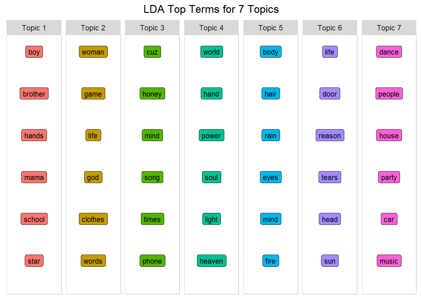
Below are a list of themes that people have labeled as potential themes in Prince's music over the years. They are tagged with certain words, and as with all topic modeling, there is overlap. But look at these manually tagged themes (listed in random order!), and see if you can find them in the model you built.
- love, time, life
- people, family
- war, peace, controversy, freedom
- pain, sad, loss
- sex, drugs
- self, society, religion
- music, dance, party
It seems that your Topic 1 is about people and family; Topic 7 is about music, dance and party; and Topic 4 is about self, society, and religion. This requires very subjective interpretation. In a business context, this step is best performed by a subject matter expert who may have an idea of what to expect. Now you can see why NLP is truly the intersection of artificial intelligence and computational linguistics!
Try running this with a different number of topics, or with just verbs, or using the raw word versus the lemmatized form, or with a different number of top words and see what insights you can derive. There are new methods to help you determine the number of topics: see the concept of perplexity here, or the
ldatuningpackage here.
Themes Over Time
Since the Prince dataset contains year, you can track the themes over time. You can be really creative here, but for now just look at a few words from two topics and view the frequency over time. Trending could be an entire tutorial in itself, so if you're really interested, check out this resource.
 p1 <-  prince_tidy %>%
  filter(!year == "NA") %>% #remove songs without years
  filter(word %in% c("music", "party", "dance")) %>%
  group_by(year) %>%
  mutate(topic_7_count = n()) %>%
  select(year, topic_7_count) %>%
  distinct() %>%
  ggplot(aes(year, topic_7_count)) + geom_smooth(se = FALSE, col = "red")

p2 <-  prince_tidy %>%
  filter(!year == "NA") %>% #remove songs without years
  filter(word %in% c("heaven","hand","soul")) %>%
  group_by(year) %>%
  mutate(topic_4_count = n()) %>%
  select(year, topic_4_count) %>%
  distinct() %>%
  ggplot(aes(year, topic_4_count)) + geom_smooth(se = FALSE)

grid.arrange(p1, p2, ncol = 2)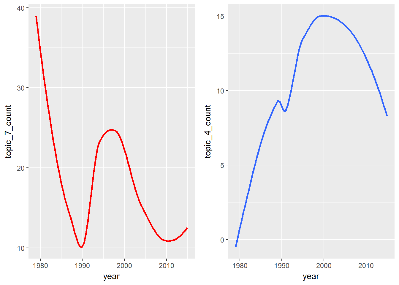
This is an extremely rudimentary example of how themes change over time, but what if you were to extend this type of analysis outside of music? Maybe your company is interested in the correlation between product sales and trending themes in customer tweets about your product. There are many applications for understanding how topics change over time.
Conclusion
This tutorial only scratches the surface of what is possible with topic modeling, NLP and machine learning. This is a burgeoning field of data science and will continue to flourish as more scientists tackle the untraversed oceans of unstructured data. In music, the concept of classifying songs based on lyrics is mostly found in research papers, so maybe you can springboard off this work and create your own contribution to the world of AI.
You used data from lyrics and nonfiction books to identify themes, classify individual documents into the most likely topics, and identify similar writers based on thematic content. Thus you were able to build a simple recommendation system based on text and labeled writers.
Keep in min; you're trying to model art with machines. An artist could say "You are the apple of my eye", but they are not referring to fruit or body parts. You have to find what is hidden. When you listen to music, you don't always hear the background vocals, but they are there. Turn up your favorite song and listen past the lead vocals and you may be surprised to find a world of hidden information. So put logic in the background and bring creativity to the forefront during your exploration!
As in all tutorials in this series, I encourage you to use the data presented here as a fun case study, but also as an idea generator for analyzing text that interests you. It may be your own favorite artists, social media, corporate, scientific, or socio-economic text. What are your thoughts about potential applications of topic modeling? Please leave a comment below with your ideas!
Stay tuned for Part Three (the fourth article) of this series: Lyric Analysis: Predictive Analytics using Machine Learning with R. There you will use lyrics and labeled metadata to predict the future of a song. You'll work with several different algorithms such as Decision Trees, Naive Bayes, and more to predict genre, decade, and possibly even whether or not a song will hit the charts! I hope to see you soon!
Caveats:
Caveat one: The only way you'll get the same results I did is if you run the code in the exact same order with the same, unmodified data files. Otherwise, reference to specific topics will not make sense.
Caveat two: There are no hard and fast rules on this work, and it is based on my own research. Although topic modeling does exist in real-world applications, there is not much activity around developing musical recommenders based entirely on lyrics.
Caveat three: Topic modeling is tricky. Building the model is one thing, but interpreting the results is challenging, subjective, and difficult to validate fully (although research is underway: see this article by Thomas W. Jones). The process is unsupervised, generative, iterative, and based on probabilities. Topics are subtle, hidden and implied and not explicit.
If you would like to learn more about machine learning using R, check out our beginner tutorial. Also, take our Introduction to Machine Learning course.
