
Introduction
In the last 10-15 years, with the progress of digital technologies, marketing strategies have changed considerably. Famous brands and smaller markets have collected a vast amount of data on transactions, customer purchases, preferences, purchasing power, buying activity, demographics, reviews, etc. All this data can help marketers understand customer behavior at different stages, from intent to buy something, to a real purchase and becoming a constant client. This is where the potential of data science comes into play.
Data science turns marketing big data into actionable insights, even if sometimes it is less intuitive at first glance, e.g., some non-evident consumer behavior patterns and co-occurrences. As a result, marketers can see a clearer picture of their target audience, attract new customers and retain the existing ones, optimize their marketing strategies, increase the company's visibility, create more successful advertising campaigns, involve new channels, and significantly maximize the company's revenue in turn.
One of the most typical data science use cases in marketing is customer churn rate prediction. Let's discuss this topic in more detail.
Data Science Use Case in Marketing: Customer Churn Rate Prediction
Customer churn is a tendency of customers to cancel their subscriptions to a service they have been using and, hence, stop being a client of that service. Customer churn rate is the percentage of churned customers within a predefined time interval. It's the opposite of the customer growth rate that tracks new clients.
Customer churn rate is a very important indicator of customer satisfaction and the overall business wellness of the company. Apart from natural churn which always takes place in any business, or seasonable churn typical of some services, there are other factors that can mean something in the company has gone wrong and should be fixed. These factors are:
- lack or low quality of customer support,
- negative customer experiences,
- switching to a competitor with better conditions or pricing strategy,
- customers’ priorities changed,
- long-time customers don’t feel satisfied,
- the service didn't meet customers’ expectations,
- finance issues,
- fraud protection on customers' payments.
High customer churn rate represents a serious problem for any company for the following reasons:
- It correlates with the company's revenue loss.
- It takes much more money to acquire new customers than to retain the existing ones. This is especially true for highly competitive markets.
- In the case of churning because of poor customer service, the company's reputation may be heavily damaged because of negative reviews left by unsatisfied ex-customers on social media or review websites.
Customer retention is a crucial component of the business strategy for all subscription-based services. To predict customer churn rate and undertake the corresponding preventive measures, it's necessary to gather and analyze the information on customer behavior (purchase intervals, the overall period of being a client, cancellations, follow-up calls and messages, online activity) and figure out which attributes and their combinations are characteristic to the clients that are at risk of leaving. Knowing in advance which customers may churn soon, especially in the case of high revenue or long-time customers, can help the company to focus exactly on them and develop an efficient strategy to try to convince them to stay. The approach can include a call to such clients with a special offer of a gift, discount, subscription upgrading for the same price, or any other customized experience.
Technically, customer churn prediction is a typical classification problem of machine learning when the clients are labeled as "yes" or "no", in terms of being at risk of churning, or not. Let's investigate this use case in Python on real-world data.
We're going to model churn in the telecom business model, where customers can have multiple services with a telecommunications company under one master agreement. The dataset contains the features of cleaned customer activity and a churn label specifying whether a customer churned or not.
Let's look at the data and explore churn rate distribution:
import pandas as pd

telcom = pd.read_csv('telco.csv')
print(f'Number of customers: {telcom.shape[0]:,}\n'
      f'Churn values: {set(telcom['Churn'])}\n\n'
      f'Churn distribution, %:\n{round(telcom.groupby(['Churn']).size()/telcom.shape[0]*100).convert_dtypes()}')
Number of customers: 7,032
Churn values: {0, 1}
Churn distribution, %:
Churn
0 73
1 27
dtype: float6427% of customers churned, which is quite a high rate. Compared to the previous data science use case, though, this dataset doesn't seem to have a severe class imbalance issue.
Now, we're going to pre-process the data for further applying machine learning techniques to perform churn prediction. This includes splitting the data into training and testing sets and extracting the features and target variables:
from sklearn.model_selection import train_test_split

target = ['Churn']
custid = ['customerID']

cols = [col for col in telcom.columns if col not in custid + target]

X = telcom[cols]
y = telcom[target]

X_train, X_test, y_train, y_test = train_test_split(X, y, test_size=0.25)
The first modeling algorithm we're going to use to predict churn labels and estimate the accuracy of the results is a simple logistic regression classification model:
from sklearn.linear_model import LogisticRegression
from sklearn.metrics import accuracy_score

lr = LogisticRegression()
lr.fit(X_train, y_train)
predictions = lr.predict(X_test)
print(f'Test accuracy: {round(accuracy_score(y_test, predictions), 4)}')
Test accuracy: 0.8009Next, let's add one more functionality to our logistic regression model, namely running it on the scaled data with L1 regularization to perform feature selection alongside the model building. Different values of the C parameter (which is the inverse of the regularization strength) have an effect on the model accuracy. For now, let's set the C value to 0.025:
lr = LogisticRegression(penalty='l1', C=0.025, solver='liblinear')
lr.fit(X_train, y_train)
predictions = lr.predict(X_test)
print(f'Test accuracy: {round(accuracy_score(y_test, predictions), 4)}')
Test accuracy: 0.7969Now, we're going to tune the C parameter for the L1 regularization to discover the optimal value which reduces the model complexity, whilst maintaining good model performance metrics. For this purpose, we'll iterate through different C values and build logistic regression instances on each, as well as calculate performance metrics.
The list C has been created in advance with the possible values of the parameter. The l1_metrics array has been built with 3 columns, with the first being the C values, and the next two being placeholders for non-zero coefficient counts and the accuracy score of the model. Let's give this approach a try:
 C  Non-Zero Coeffs  Accuracy
0  1.0000             23.0  0.801479
1  0.5000             22.0  0.799204
2  0.2500             21.0  0.802048
3  0.1000             20.0  0.802617
4  0.0500             18.0  0.802048
5  0.0250             13.0  0.796928
6  0.0100              5.0  0.790102
7  0.0050              3.0  0.783276
8  0.0025              2.0  0.745734
We can see that lower C values shrink the number of non-zero coefficients (i.e., features for modeling) reducing the model complexity, but they also decrease the model accuracy. It seems that the C value of 0.05 is the optimal one: it reduces the number of features to 18 while giving the accuracy score slightly higher than the one in the non-regularized model.
Now, let's try another modeling algorithm – the decision tree model:
from sklearn.tree import DecisionTreeClassifier

clf = DecisionTreeClassifier()
clf.fit(X_train, y_train)
predictions = clf.predict(X_test)
print(f'Test accuracy: {round(accuracy_score(y_test, predictions), 4)}')
Test accuracy: 0.7275To select a more precise model while avoiding overfitting, we can try tuning tree depth (the max_depth parameter) and identify its optimal value. Technically, the process is very similar to the one for selecting the optimal C parameter of the logistic regression model above: here, we'll iterate through multiple values of the max_depth parameter, fit a decision tree for each, and then calculate performance metrics.
The list depth_list has been created in advance with the possible values of the parameter. The depth_tuning array has been built with 2 columns, with the first one being filled with the depth candidates, and the other being a placeholder for the accuracy score. Let's apply this approach and find the optimal tree depth:
depth_list = list(range(2, 15))
depth_tuning = np.zeros((len(depth_list), 2))
depth_tuning[:, 0] = depth_list

for index in range(len(depth_list)):
    clf = DecisionTreeClassifier(max_depth=depth_list[index])
    clf.fit(X_train, y_train)
    predictions = clf.predict(X_test)
    depth_tuning[index, 1] = accuracy_score(y_test, predictions)

col_names = ['Max_Depth', 'Accuracy']
print(pd.DataFrame(depth_tuning, columns=col_names))
Max_Depth Accuracy
0 2.0 0.756542
1 3.0 0.783276
2 4.0 0.782708
3 5.0 0.791809
4 6.0 0.778157
5 7.0 0.780432
6 8.0 0.757110
7 9.0 0.762230
8 10.0 0.763936
9 11.0 0.752560
10 12.0 0.745165
11 13.0 0.732651
12 14.0 0.727531Hence, the accuracy score first increases with more depth and then starts to decline. At the max_depth of 5, the tree shows the highest accuracy score, hence we can consider this value as the optimal tree depth.
After identifying the best parameter values for both logistic regression and decision tree models, let's reconstruct those models and then detect and interpret the main factors that are driving churn to go up or down.
For the logistic regression model, we're going to extract and explore the exponents of the resultant coefficients:
# Reconstructing the best model
lr = LogisticRegression(penalty='l1', C=0.05, solver='liblinear')
lr.fit(X_train, y_train)
predictions = lr.predict(X_test)

# Combining feature names and coefficients into one dataframe
feature_names = pd.DataFrame(X_train.columns, columns=['Feature'])
log_coef = pd.DataFrame(np.transpose(lr.coef_), columns=['Coefficient'])
coefficients = pd.concat([feature_names, log_coef], axis=1)

# Calculating exponents of the coefficients
coefficients['Exp_Coefficient'] = np.exp(coefficients['Coefficient'])

# Removing coefficients that are equal to zero
coefficients = coefficients[coefficients['Coefficient']!=0]
print(coefficients.sort_values(by=['Exp_Coefficient']))
Feature Coefficient Exp_Coefficient
21 tenure -0.907750 0.403431
4 PhoneService_Yes -0.820517 0.440204
17 Contract_Two year -0.595271 0.551413
8 TechSupport_Yes -0.418254 0.658195
16 Contract_One year -0.414158 0.660896
5 OnlineSecurity_Yes -0.412228 0.662173
6 OnlineBackup_Yes -0.143100 0.866667
3 Dependents_Yes -0.039299 0.961463
7 DeviceProtection_Yes -0.017465 0.982687
11 PaperlessBilling_Yes 0.071389 1.073999
1 SeniorCitizen_Yes 0.097904 1.102857
19 PaymentMethod_Electronic check 0.188533 1.207477
22 MonthlyCharges 0.901454 2.463182We can see that the feature with the largest effect on the odds of churning is tenure. In general, the coefficient exponents lower than 1 decrease the odds, while those higher than 1 increase them.
For the decision tree model, we're going to extract and plot the if-else rules:
# Reconstructing the best model
clf = DecisionTreeClassifier(max_depth=5)
clf.fit(X_train, y_train)
predictions = clf.predict(X_test)

from sklearn import tree
import graphviz

# Exporting a graphviz object from the trained decision tree
exported = tree.export_graphviz(decision_tree=clf,
                                out_file=None,
                                feature_names=cols,
                                precision=1,
                                class_names=['Not churn', 'Churn'],
                                filled=True)
graph = graphviz.Source(exported)
display(graph)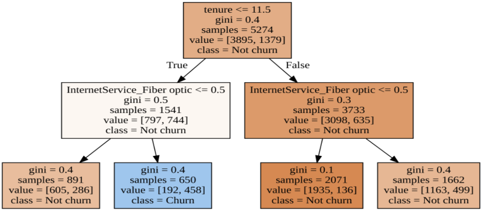
We obtained a good-looking decision tree visualization that can be interpreted as a set of if-else rules starting from the top. Again we see that customer tenure is the most important variable driving churn. The decision tree can be built with more layers, and this will give more insights into other variables.
As potential ways forward, we can try further adjusting the model parameters, using different approaches of train/test splitting, applying and comparing other machine learning algorithms, and analyzing various score types to estimate the model performance.
If you’re curious to dive deeper into customer churn rate prediction and other applications of data science in marketing, this course on Machine Learning for Marketing in Python can be a good place to start.