HomeCheat sheetsR Programming

xts Cheat Sheet: Time Series in R

Get started on time series in R with this xts cheat sheet, with code examples.
Jul 2021  · 5 min read

Even though the data.frame object is one of the core objects to hold data in R, you'll find that it's not really efficient when you're working with time series data. You'll find yourself wanting a more flexible time series class in R that offers a variety of methods to manipulate your data.

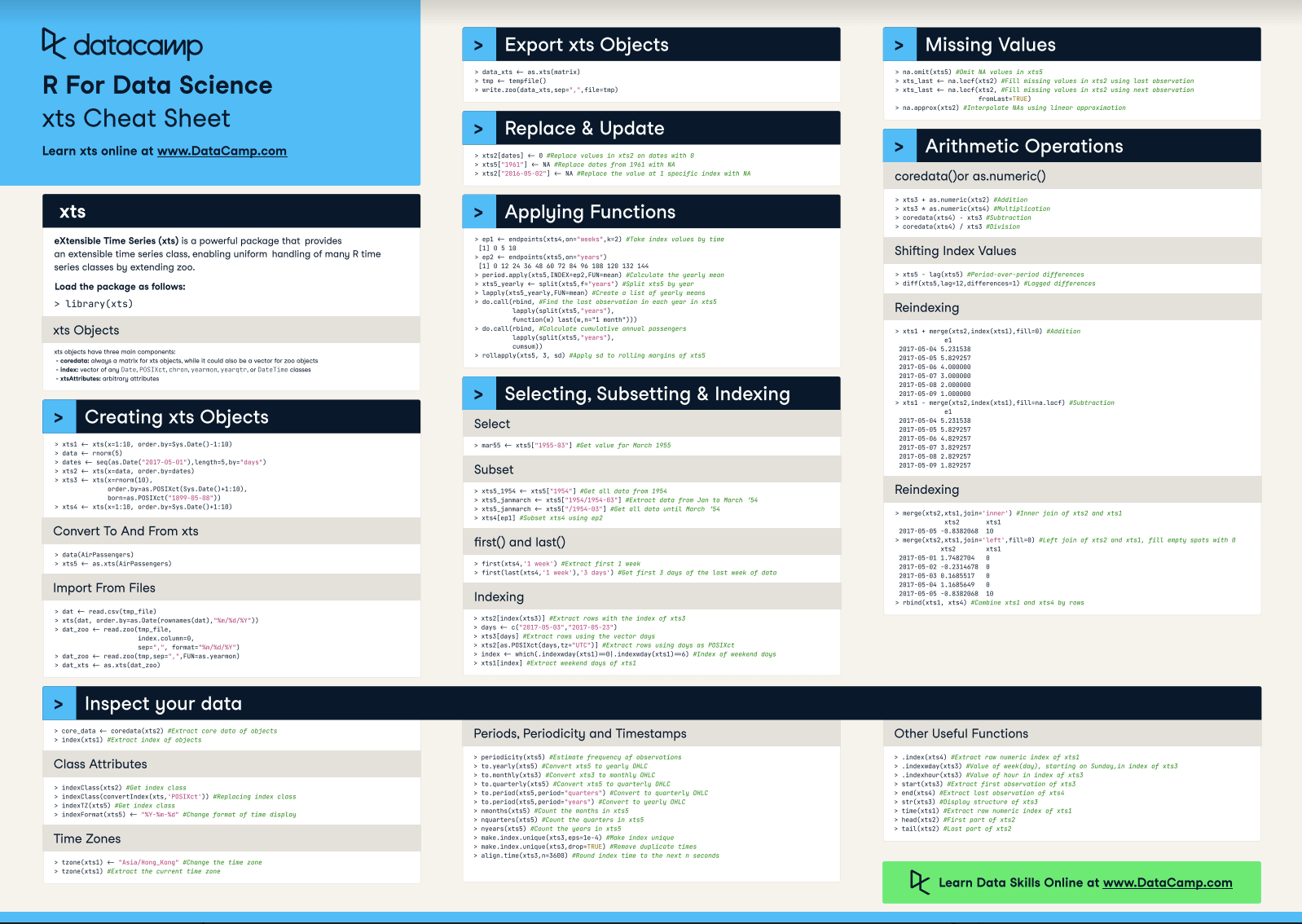
 xts  or the Extensible Time Series is one of such packages that offers such a time series object. It's a powerful R package that provides an extensible time series class, enabling uniform handling of many R time series classes by extending zoo, which is the package that is the creator for an S3 class of indexed totally ordered observations which includes irregular time series.

xts has a lot to offer to make your time series analysis fast and mistake free, but it can take some time to get used to it. 

This xts cheat sheet provides you not only with an overview of the xts object, how to create and inspect them, but also goes deeper into how you can manipulate time series with xts: you'll see how to replace and update values, how to select, index and subset your objects, how to handle missing values and how to perform arithmetic operations.

Click on the button below to see (and download) the xts cheat sheet: 

Have this cheat sheet at your fingertips

Download PDF

This cheat sheet will help you to get yourself up to speed in no time! 

R For Data Science Cheat Sheet: xts

eXtensible Time Series (xts) is a powerful package that provides an extensible time series class, enabling uniform handling of many R time series classes by extending zoo.

Load the package as follows:

library(xts)

Xts Objects

xts objects have three main components:

  • coredata: always a matrix for xts objects
  • index: vector of any Date, POSIXct, chron, yearmon, yearqtr, or DateTime classes
  • xtsAttributes: arbitrary attributes

Creating xts Objects

xts1 <- xts(x=1:10, order.by=Sys.Date()-1:10)
data <- rnorm(5)
dates <- seq(as.Date("2017-05-01"), length=5, by="days")
xts2 <- xts(x=data, order.by=dates)
xts3 <- xts(x=rnorm(10), order.by=as.POSIXct(Sys.Date()+1:10), born=as.POSIXct("1899-05-08")
xts4 <- xts(x=1:10, order.by=Sys.Date()+1:10)

Convert To And From xts

data(AirPassengers)
xts5 <- as.xts(AirPassengers)

Import From Files

dat <- read.csv(tmp_file)
xts(dat, order.by=as.Date(rownames(dat),"%m/%d/%Y"))
dat_zoo <- read.zoo(tmp_file, index.column=0, sep=",", format="%m/%d/%Y")
dat_zoo <- read.zoo(tmp,sep=",",FUN=as.yearmon)
dat_xts <- as.xts(dat_zoo)

Inspect Your Data

Extract core data of objects

core_data <- coredata(xts2)

Extract index from objects

index(xts1)

Class Attributes

Get index class

indexClass(xts2)

Replacing index class

indexClass(convertIndex(xts,'POSIXct'))

Get index class

indexTZ(xts5)

Change format of time display

indexFormat(xts5) <- "%Y-%m-%d"

Time Zones

Change the time zone

tzone(xts1) <- "Asia/Hong_Kong"

Extract the current time zone

tzone(xts1)

Periods, Periodicity & Timestamps

Estimate frequency of observations

periodicity(xts5)

Convert xts5 to yearly OHLC

to.yearly(xts5)

Convert xts3 to monthly OHLC

to.monthly(xts3)

Convert xts5 to quarterly OHLC

to.quarterly(xts5)

Convert to quarterly OHLC

to.period(xts5,period="quarters")

Convert to yearly OHLC

to.period(xts5,period="years")

Count the months in xts5

nmonths(xts5)

Count the quarters in xts5

nquarters(xts5)

Count the years in xts5

nyears(xts5)

Make index unique

make.index.unique(xts3,eps=1e-4)

Remove duplicate times

make.index.unique(xts3,drop=TRUE)

Round index time to the next n seconds

align.time(xts3, n=3600)

Other Useful Functions

Extract raw numeric index of xts1

.index(xts4)

value of weekday in index of xts3

.indexwday(xts3)

Value of hour in index of xts3

.indexhour(xts3)

Extract first observation of xts3 

start(xts3)

Extract last observation of xts4 

end(xts4)

Display structure of xts3 

str(xts3)

Extract raw numeric index of xts1

time(xts1)

First part of xts2

head(xts2)

Last part of xts2 

tail(xts2)

Export xts Objects

data_xts <- as.xts(matrix)
tmp <- tempfile()
write.zoo(data_xts,sep=",",file=tmp)

Replace & Update

Replace values in xts2 on dates with 0 

xts2[dates] <- 0 

Replace dates from 1961 with NA 

xts5["1961"] <- NA

Replace the value at 1 specific index with NA

 xts2["2016-05-02"] <- NA  
  

Applying Functions

Locate endpoints by time 

ep1 <- endpoints(xts4,on="weeks",k=2)  
ep2 <- endpoints(xts5,on="years")

Calculate the yearly mean 

period.apply(xts5,INDEX=ep2,FUN=mean)

Split xts5 by year

xts5_yearly <- split(xts5,f="years")

Create a list of yearly means   

lapply(xts5_yearly,FUN=mean) 

Find the last observation in each year in xts5

do.call(rbind,  lapply(split(xts5,"years"), function(w) last(w,n="1 month")))

Calculate cumulative annual passengers

do.call(rbind,  lapply(split(xts5,"years"),  cumsum))

Apply standard deviation to rolling margins of xts5

rollapply(xts5, 3, sd) 

Selecting, Subsetting & Indexing

Select

mar55 <- xts5["1955-03"] #Get value for March 1955

Subset

Get all data from 1954 

xts5_1954 <- xts5["1954"] 

Extract data from Jan to March ‘54 

xts5_janmarch <- xts5["1954/1954-03"]

Get all data until March ‘54  

xts5_janmarch <- xts5["/1954-03"] 

Subset xts4 using ep2 

xts4[ep1]

first() and last()

first(xts4,'1 week') #Extract first 1 week
first(last(xts4,'1 week'),'3 days') #Get first 3 days of the last week of data

Indexing

Extract rows with the index of xts3 

xts2[index(xts3)] 

Extract rows using the vector days 

days <- c("2017-05-03","2017-05-23") 
xts3[days]

Extract rows using days as POSIXct 

xts2[as.POSIXct(days,tz="UTC")] 

Index of weekend days

index<-which(.indexwday(xts1)==0|.indexwday(xts1)==6) 

Extract weekend days of xts1 

xts1[index]

Missing Values

Omit NA values in xts5 

na.omit(xts5)

Fill missing values in xts2 using last observation

xts_last <- na.locf(xts2)

Fill missing values in xts2 using next observation

xts_last <- na.locf(xts2,  fromLast=TRUE)

Interpolate NAs

na.approx(xts2) 

Arithmetic Operations

coredata() or as.numeric()

xts3 + as.numeric(xts2) #Addition
xts3 * as.numeric(xts4) #Multiplication
coredata(xts4) - xts3 #Subtraction
coredata(xts4) / xts3 #Division

Shifting Index Values

Period-over-period differences 

xts5 - lag(xts5)

Lagged differences

diff(xts5,lag=12,differences=1) 

Reindexing

xts1 + merge(xts2,index(xts1),fill=0) #Addition
xts1 - merge(xts2,index(xts1),fill=na.locf) #Subtraction

Merging

merge(xts2,xts1,join='inner') # Inner join of xts2 and xts1
merge(xts2,xts1,join='left',fill=0) #Left join of xts2 and xts1,
rbind(xts1, xts4)

Going Further

Want to know more about xts? Check out DataCamp's Manipulating Time Series Data in R with xts & zoo course! 

Topics
Related

Data Science in Finance: Unlocking New Potentials in Financial Markets

Discover the role of data science in finance, shaping tomorrow's financial strategies. Gain insights into advanced analytics and investment trends.
 Shawn Plummer's photo

Shawn Plummer

9 min

5 Common Data Science Challenges and Effective Solutions

Emerging technologies are changing the data science world, bringing new data science challenges to businesses. Here are 5 data science challenges and solutions.
DataCamp Team's photo

DataCamp Team

8 min

Navigating R Certifications in 2024: A Comprehensive Guide

Explore DataCamp's R programming certifications with our guide. Learn about Data Scientist and Data Analyst paths, preparation tips, and career advancement.
Matt Crabtree's photo

Matt Crabtree

8 min

A Data Science Roadmap for 2024

Do you want to start or grow in the field of data science? This data science roadmap helps you understand and get started in the data science landscape.
Mark Graus's photo

Mark Graus

10 min

R Markdown Tutorial for Beginners

Learn what R Markdown is, what it's used for, how to install it, what capacities it provides for working with code, text, and plots, what syntax it uses, what output formats it supports, and how to render and publish R Markdown documents.
Elena Kosourova 's photo

Elena Kosourova

12 min

Introduction to DynamoDB: Mastering NoSQL Database with Node.js | A Beginner's Tutorial

Learn to master DynamoDB with Node.js in this beginner's guide. Explore table creation, CRUD operations, and scalability in AWS's NoSQL database.
Gary Alway's photo

Gary Alway

11 min

See MoreSee More