Course
Time Series Analysis in R
4 hr
61.2K
Time Series is the measure, or it is a metric which is measured over the regular time is called as Time Series. Time Series Analysis example are Financial, Stock prices, Weather data, Utility Studies and many more.
The time series model can be done by:
In this tutorial, you will be given an overview of the stationary and non-stationary time series models. You will be shown how to identify a time series by calculating its ACF and PACF. The figures of these functions make it possible to judge the stationarity of a time series. We can make a non-stationary series stationary by differentiating it. Knowing the nature of a series, it is now easy to predict future values from a model that the series follows. An illustration of real data that can be found in the TSA package of R will also be part of this tutorial.
Let $X$ be a random variable indexed to time (usually denoted by $t$), the observations $\left\{x_t,\,t\in \textbf{N}\right\}$ is called a time series. $\textbf{N}$ is the integer set which is considered here as the time index set. $N$ can also be a timestamp. Stationarity is a critical assumption in time series models, and it implies homogeneity in the series that the series behaves in a similar way regardless of time, which means that its statistical properties do not change over time. There are two forms of stationarity: strong and week forms.
A stationary process $\left\{x_t,\,t\in \textbf{N}\right\}$ is said to be strictly or strongly stationary if its statistical distributions remain unchanged after a shift o the time scale. Since the distributions of a stochastic process are defined by the finite-dimensional distribution functions, we can formulate an alternative definition of strict stationarity. If in every $n$, every choice of times $t_1, t_2, \ldots, t_n\in \textbf{N}$ and every time lag $k$ such that $t_{i+k}\in\textbf{N}$, the $n$-dimensional random vector $(X_{t_1+k}, X_{t_2+k}, \ldots, X_{t_n+k})$ has the same distribution as the vector $(X_{t_1}, X_{t_2}, \ldots, X_{t_n})$, then the process is strictly stationary. That is for $h$ and $x_i$
\begin{align*} P(X_{t_1}\leq x_1, X_{t_2}\leq x_2, \ldots, X_{t_k}\leq x_k) &= F(x_{t_1}, x_{t_2}, \ldots, x_{t_k})\\ &= F(x_{h+t_1}, x_{h+t_2}, \ldots, x_{h+t_k})\\ &= P(X_{h+t-1}\leq x_1, X_{h+t_2}\leq x_2, \ldots, X_{h+t_k}\leq x_k) \end{align*}
for any time shift $h$ and observation $x_j$. If $\left\{X-t,\,t\in\textbf{N}\right\}$ is strictly stationary, then the marginal distribution of $X_t$ is independent of $t$. Also,the two-dimensional distributions of $(X_{t_1}, X_{t_2})$ are independent of the absolute location of $t_1$ and $t_2$, only the distance $t_1-t_2$ matters. As a consequence, the mean function $E(X)$ is constant, and the covariance $Cov(X_t,X_{t-k})$ is a function of $k$ only, not of the absolute location of $k$ and $t$. At higher order moments, like the third order moment, $E[X_uX_tX_v]$ remains unchanged if one add a constant time shift to $s, t, u$.
A univariate time series $X_t$ is stationary if its mean, variance and covariance are independent of time. Thus, if $X_t$ is a time series (or stochastic process, meaning random variables ordered in time) that is defined for $t=1,2,3,\ldots, n$ and for $t=0, -1, -2, -3, \ldots$, then, $X_t$ is mathematically weakly stationary if
\begin{align} (i) & E[X_t] = \mu\\ (ii) & E\left[(X-\mu)^2\right] = Var(X_t) = \gamma(0) = \sigma^2\\ (iii) & E\left[(X_t-\mu)(X_{t-k}-\mu)\right] = Cov(X_t, X_{t-k}) = \gamma(k) \end{align}
The first two conditions ($(i)$ and $(ii)$) require the process to have constant mean and variance respectively, while $(iii)$ requires that the covariance between any two values (formally called covariance function) depends only on the time interval $k$ between these two values and not on the point in time $t$.
If a process is Gaussian with finite second moments, then weak stationarity is equivalent to strong stationarity. Strick stationarity implies weak stationarity only if the necessary moments exist. Strong stationarity also requires distributional assumptions. The strong form is generally regarded as too strict, and therefore, you will mainly be concerned with weak stationarity, sometimes known as covariance stationarity, wide-sense stationarity or second order stationarity.
A time series, in which the observations fluctuate around a constant mean, have continuous variance and stochastically independent, is a random time series. Such time series doesn't exhibit any pattern:
An example of a stationary random model can be written as
$$X_t = \mu+\varepsilon_t$$ where $\mu$ is a constant mean such that $E[X_t] = \mu$ and $\varepsilon_t$ is the noise term assumed to have a zero mean, constant variance and are independent (also known as white noise).
# purely random process with mean 0 and standard deviation 1.5
eps <- rnorm(100, mean = 0, sd = 1)
mu <- 2 # the constant mean
# The process
X_t <- mu + eps

# plotting the time series
ts.plot(X_t, main = "Example of (random) stationary time series", ylab = expression(X[t]))
The simulated process fluctuates around the constant mean $\mu = 2$.
The theoretical auto-covariance function (ACF) of a stationary stochastic process is an important tool for assessing the properties of times series. Let $X_t$ be a stationary stochastic process with mean $\mu$ and variance $\sigma^2$. The ACF at lag $k$, $\gamma(k)$, is $$\gamma(k) = \frac{\gamma(k)}{\gamma(0)} = \frac{\gamma(k)}{\sigma^2}$$
The ACF function is a normalized measure of the auto-covariance and possesses several properties.
The ACF of the above process is represented by the following figure.
# Auto-covariance function of the simulated stationary random time series
acf(X_t, main = "Auto-covariance function of X")
Note 1. The lack of uniqueness is a characteristic of the ACF. Even if a given random has a unique covariance structure, the opposite is generally not true: it is possible to find more than one stochastic process with the same ACF. This causes specification problems is illustrated in [@jenkinsd].
Note 2: A very special matrix is obtained by the autocorrelation function of a stationary process. It is called the Toeplitz matrix. It is a kind of variance and covariance matrix of order $m = t-k$ (the lag, including auto-correlations to lag $m-1$), so it is diagonal, symmetric, positive definite.
\begin{equation} \begin{pmatrix} 1 & \rho(1) & \rho(2) & \cdots & \rho(m-1)\\ \rho(1) & 1 & \rho(1) & \cdots & \rho(m-2)\\ \cdots &\cdots &\cdots &\cdots &\cdots\\ \rho(m-1) & \rho(m-2) & \cdots & \rho(1) & 1 \end{pmatrix} \end{equation}
A discrete process $\left\{Z_t\right\}$ is called a purely random process if the random variables $Z_t$ form a sequence of mutually independent and identically distributed (i.i.d.) variables. The definition implies the process has constant mean and variance.
$$\gamma(k) = cov(Z_t, Z_{t+k}) = 0,\quad\forall k\in -3,-2,-1,0,1,2,3, \ldots$$ Given that the mean and the autocovariance function (acvf) do not depend on time, the process is second-order stationary.
A process $\left\{X_t\right\}$ is said to be a random walk process if $X_t = X_{t-1}+Z_t$, with $Z_t$ a purely random process with mean $\mu$ and variance $\sigma^2_Z$. The process is usually stating at $t = 0$ and we have $X_1 = Z_0$ which means that $X_0 = 0$. We have
\begin{align*} X_1 &= X_0 + Z_1, \quad\text{at } t = 1\\ X_2 &= X_1 + Z_2 = X_0 + Z_1+ Z_2, \quad\text{at } t = 2\\ X_3 &= X_2 + Z_3 = X_0 + Z_1+ Z_2 + Z_3, \quad\text{at } t = 3\\ &\cdots\\ X_t &= X_0 + \sum_{i = 1}^tZ_i \end{align*}
The first order moment (or the expected value) for this process is equal to $$E[X_t] = X_0 +\sum_{i = 1}^tE[Z_i] = X_0 + t\mu_z = t\mu_z$$ and the variance $$Var(X_t) = t\sigma^2_Z$$ Note that the mean and variance change with time, so, the process is \textbf{non-stationary}. An example of time series behaving like random walks is share prices.
# seed X_0 = 0
X <- 0

# purely random process with mean 0 and standard deviation 1.5
Z <- rnorm(100, mean = 0.5, sd = 1.5)

# the process
for (i in 2:length(Z)){
  X[i] <- X[i-1] + Z[i]
}

# process plotting
ts.plot(X, main = "Random walk process")Differencing is the most common method for making a time series data stationary. This is a special type of filtering, particularly important in removing a trend. For seasonal data, first order differencing data is usually sufficient to attain stationarity in a mean. Let $X_t = \left\{X_1, X_2,\ldots, X_n\right\}$ be non-stationary time series. The stationary tie is obtained as
$$\Delta X_{t+1} = X_{t+1}-X_t\quad\text{or }\,\Delta X_{t} =X_t-X_{t-1}$$ which is simply called the first-order difference. If the second-order difference is required, you can use the operator $\Delta^2$ is the difference of first-order differences
$$\Delta^2X_{t+2} = \Delta X_{t+2} - \Delta X_{t+1}$$
# differencing and plotting of the random walk process
ts.plot(diff(X))
You know that the resulting first order difference fluctuates around a constant mean 0. This is because mathematically
$$\Delta X_{t+1} = X_{t+1}-X_t = Z_t$$ which is stationary because it's a purely random process with constant mean and constant variance.
Let $\left\{Z_t\right\}$ be a purely random process with mean zero and variance $\sigma^2_Z$. The process is said to be a Moving Average of order #q# if
$$X_t = \beta_0Z_t-\beta_1Z_{t-1}-\cdots-\beta_q Z_{t-q}$$ where $\beta_i,\, i = 1,2,\ldots,q$ are constants. The random variables $Z_t, \,t\in\textbf{N}$ are usually scaled so that $\beta_0=1$
# purely random process with mean 0 and standard deviation 1.5 (arbitrary choice)
Z <- rnorm(100, mean = 0, sd = 1.5)

# process simulation
X <- c()
for (i in 2:length(Z)) {
  X[i] <- Z[i] - 0.45*Z[i-1]
}

# process plotting
ts.plot(X, main = "Moving Average or order 1 process")
For the MA(1) process, the 3 conditions can be verified as follows:
\begin{align} E[X_t] &= 0\\ Var(X_t) &= E[X_t^2] - 0 = E\left[Z_t^2-2\beta Z_tZ_{t-1}+\beta^2Z_{t-1}^2\right]= \sigma^2_Z+\beta^2\sigma^2_Z\\ \gamma(k) &= cov(X_t, X_{t+k}) = E[X_tX_{t+k}] - E[X_t]E[X_{t+k}] = E[X_tX_{t+k}]\\ &= E\left[(Z_t-\beta Z_{t-1})(Z_{t+k}-\beta Z_{t-1+k})\right]\\ &= E\left[Z_tZ_{t+k} - \beta Z_tZ_{t-1+k} -\beta Z_{t-1}Z_{t+k} + \beta^2 Z_{t-1}Z_{t-1+k}\right]\\ \end{align}
for $k = 0,\, \gamma(0) = Var(X_t) = \sigma^2_Z(1+\beta^2)$
for $k = 1,\, \gamma(1) = E\left[Z_tZ_{t+1} - \beta Z_t^2 -\beta Z_{t-1}Z_{t+1} + \beta^2 Z_{t-1}Z_{t}\right] = -\beta\sigma^2_Z$
and for $k>1,\, \gamma(k) = 0.$
Thus, the MA(1) process has a covariance of zero when the displacement is more than one period. That is it has a memory of only one period.
The ACF for MA(1) is therefore
$$\rho(k) = \frac{\gamma(k)}{\gamma(0)} = \begin{cases}1, &\text{k }=0\\\frac{-\beta}{1+\beta^2}, & \text{k }\pm 1\end{cases}$$
Question: redo the work for MA(2)
It can be seen why the sample autocorrelation function can be useful in specifying the order of a moving average process: the autocorrelation functionï²(k) for the MA(q) process has q non-zero values (significantly different from zero) and is zero for $k > q$. No restrictions on $\left\{\beta_i\right\}$ are required for MA to be stationary. However, $\left\{\beta_i\right\}$ have to be restricted to ensure invertibility.
Let $\left\{Z_t\right\}$ be a purely random process with mean zero and variance $\sigma_Z^2$. A process $\left\{X_t\right\}$ will be called an autoregressive process of order $p$ if $$X_t = \alpha_1X_{t-1}+\alpha_2X_{t-2}+\cdots+\alpha_pX_{t-p}+Z_t$$ In the autoregressive process of order $p$, the current observation $X_t$ (today's return for instance) is generated by a weighted average of past observations going back $p$ periods, together with a random independent variables but on past values of $X_t$ and hence autoregressive. These types of processes were introduced by [@greenwood1920inquiry]. The AR($p$) above can be written with a constant mean
$$X_t = \delta+\alpha_1X_{t-1}+\alpha_2X_{t-2}+\cdots+\alpha_pX_{t-p}+Z_t$$ where $\mu$ is a constant term which relates to being the mean of the time series and $\alpha_1, \alpha_2,\ldots, \alpha_p$ can be positive or negative. The AR($p$) is stationary if $E[X_t] = E[X_{t-1}] = \cdots = E[X_p] = \mu$. Thus,
\begin{align*} E[X_t] = \mu &= \delta + \alpha_1\mu+\alpha_2\mu+\cdots+\alpha_p\mu+ 0\\ \Rightarrow \mu &= \frac{\delta}{1-\alpha_1-\alpha_2-\cdots-\alpha_p} \end{align*} For the last formulate to be a constant, we consider the condition $\alpha_1+\alpha_2+\cdots+\alpha_p<1$.
</1>
Consider the case when $p=1$, then $$X_t = \alpha X_{t-1}+Z_t$$ is the first order autoregressive AR(1) which is also known as Markov process. Using the backshift operator $BX_t = X_{t-1}$, you can express AR(1) as an infinite MA process. We have $$(1 - \alpha B)X_t = Z_t$$ so, \begin{align*} X_t &= \frac{Z_t}{1-\alpha B}\\ &= (1+\alpha B +\alpha^2B^2+ \cdots)Z_t\\ &=Z_t+\alpha Z_{t-1}+\alpha^2Z_{t-2}+\cdots\\ &=Z_t+\beta_1 Z_{t-1}+\beta_2 Z_{t-2}+\cdots\\ \end{align*}
Then $E[X_t] = 0$ and $Var(X_t) = \sigma^2_Z(1+\alpha^2+\alpha^4+\cdots)$. The series converges with the condition $|\alpha|<1$.
Question: Given that an AR(1) process $X_t = \alpha_1X_1+Z_t$ is a purely random process with mean zero and variance $\sigma^2_Z$ and $\alpha$ is a constant with necessary conditions on $\alpha$, derive the variance and auto-covariance function of $X_t$.
# constant alpha
alpha = 0.5
# purely random process with mean 0 and standard deviation 1.5
Z <- rnorm(100, mean = 0, sd = 1.5)
# seed
X <- rnorm(1)
# the process
for (i in 2:length(Z)) {
X[i] <- 0.7*X[i-1]+Z[i]
}
# process plotting
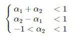
ts.plot(X)Question: Express the stationary condition of the AR (2) model regarding parameter values. That is, show the following conditions:
You can also express an AR process of finite order, say p, as an MA process of infinite order. This can be done by successive substitution or by using the backward shift operator.
In model building, it may be necessary to mix both AR and MA terms in the model. This leads to mixed autoregressive â moving averages (ARMA) process. An ARMA process which contains $p$ autoregressive terms and $q$ moving average terms is said to be of order $(p, q)$ and is given by
$$X_t = \alpha_1X_{t-1}+\alpha_2X_{t-2}+\cdots+\alpha_pX_{t-p}+Z_t-\beta_1Z_{t-1}-\beta_2Z_{t-2}-\cdots-\beta_qZ_{t-q}$$ Using the backshift operator B, the equation can be written as
$$\alpha_p(B)X_t = \beta_q(B)Z_t$$ where $\alpha_p(B)$ and $\beta_q(B)$ are polynomials of order $p$ and $q$ respectively, such that
\begin{align*} \alpha_p(B) &= \left(1-\alpha_1 B-\cdots-\alpha_p B^p\right)\\ \beta_q(B) &= \left(1-\beta_1 B-\cdots-\beta_p B^p\right) \end{align*}
For the process to be invertible, roots of $\beta_q(B)$ must lie outside a unit circle. To be stationary, we require the roots of $\alpha_p(B)=0$ to lie outside a unit circle. It's also assumed $\alpha_p(B)=0$ and $\beta_q(B) = 0$ share no common roots.
This process is of order $(1,1)$ and is given by the equation $$X_t = \alpha_1X_{t-1}+Z_t-\beta_1Z_{t-1}$$
with the conditions $|\alpha_1|<1$ and $|\beta_1|<1$ is needed for stationarity and invertibility proof. When $\alpha < 0$, the ARMA(1,1) reduces to MA(1) and when $\beta_1<0$, we'll have an AR(1). An ARMA(1,1) process can be transformed into a pure autoregressive representation using backshift operator:
$$(1-\alpha_1B)X_t = (1-\beta_1B)Z_t$$
We have
\begin{align*} \frac{1-\alpha_1B}{1-\beta_1B}X_t &= Z_t\\ \pi(B)X_t &= Z_t \end{align*}
with
\begin{align*} \pi(B) = 1-\pi_1B-\pi_2B^2-\ldots &= \frac{1-\alpha_1B}{1-\beta_1B}\\ (1-\beta_1B)(1-\pi_1B-\pi_2B^2-\ldots) &= 1-\alpha_1B\\ 1-\left[(\pi_1+\beta_1)B - (\pi_2+\beta_2)B^2 - (\pi_3+\beta_3)B^3\right] & = 1-\alpha_1B \end{align*}
By identification of B's coefficients on both sides of the equation, we get the unknown terms as $$\pi_j = \beta_1^{j-1}(\alpha_1-\beta_1),\,\text{for }\, j\geq1$$
The expectation of $X_t$ is given by $E[X_t] = \alpha_1E[X_{t-1}]$ and under stationarity assumption, we have $E[X_t] = E[X_{t-1}] = \mu = 0$. This is useful for the calculation of the auto-covariance function which is obtained as follows:
For $k = 0$,
\begin{align*} \gamma(1)&=\alpha_1\gamma(0)+E\left[X_{t-1}Z_t\right]-\beta_1E\left[X_{t-1}Z_{t-1}\right]\\ &=\alpha_1\left(\alpha_1\gamma(1)+ \sigma^2_Z - \beta_1(\alpha_1-\beta_1)\sigma^2_Z\right)-\beta_1\sigma^2_Z\\ &= \alpha^2\gamma(1)+(\alpha_1-\beta_1)(1-\alpha_1\beta_1)\sigma^2_Z\\ \Rightarrow \gamma(1)&=\frac{(\alpha_1-\beta_1)(1-\alpha_1\beta_1)\sigma^2_Z}{1-\alpha^2}\\ \Rightarrow \gamma(0)&=\alpha_1\frac{(\alpha_1-\beta_1)(1-\alpha_1\beta_1)\sigma^2_Z}{1-\alpha^2}+ \sigma^2_Z - \beta_1(\alpha_1-\beta_1)\sigma^2_Z\\ &=\frac{\left(1+\beta_1^2-2\alpha_1\beta_1\right)\sigma_Z^2}{1-\alpha^2} \end{align*}
For $k \geq 2$,
\begin{align*} \gamma(2)&=\alpha_1\gamma(k-1) \end{align*}
Hence, the ACF of ARMA(1,1) is:
$$\rho(k) = \begin{cases} 1, &\text{for }\,k=0\\ \frac{(\alpha_1-\beta_1)(1-\alpha_1\beta_1)}{1+\beta_1^2-2\alpha_1\beta_1},&\text{for }\,k=1\\ \alpha_1\rho(k-1), &\text{for }\,k\geq2\\ \end{cases} $$ The ACF of ARMA(1,1) combines the characteristic of both AR(1) and MA(1) processes. The MA(1) and AR(1) parameters are both present in $\rho(1)$. Beyond $\rho(1)$, the ACF of an ARIMA(1,1) odel follows the same pattern as the ACF of an AR(1).
Question: Find the partial autocorrelation function (PACF) of ARMA(1,1) process.
Note: A characteristic of time series processes are given in terms of their ACF and PACF. The most crucial steps in time series analysis, identify and build a model based on the available data, where the ACF and PACF are unknown.
# purely random process with mean 0 and standard deviation 1.5
Z <- rnorm(100, mean = 0, sd = 1.5)

# Process
X <- rnorm(1)

for (i in 2:length(Z)) {
  X[i] <- 0.35*X[i-1] + Z[i] + 0.4*Z[i-1]
}

# process plotting
ts.plot(X, main = "ARMA(1,1) process")

# ACF et PACF
par(mfrow = c(1,2))
acf(X); pacf(X)Autoregressive Integrated Moving Average Models are time series defined by the equation:
In this section, you will use real-time series to fit the optimal model from it. For that purpose, you'll use the forecast package. The function auto.arima fits and selects the optimal model from the data and forecast function allows the prediction of h periods ahead.
# R packages to be used
library(forecast)
library(TSA)
Example 1:
# Data from TSA package
data("co2")
data("boardings")

# fitting
fit <- auto.arima(co2)

# Time series plot
plot(fc <- forecast(fit, h = 15))
Example 2:
data("boardings")

# fitting
fit2 <- auto.arima(boardings[,"log.price"])

# forecasting
plot(fc2 <- forecast(fit2, h = 15))Greenwood, Major, and G Udny Yule. 1920. “An Inquiry into the Nature of Frequency Distributions Representative of Multiple Happenings with Particular Reference to the Occurrence of Multiple Attacks of Disease or of Repeated Accidents.” Journal of the Royal Statistical Society 83 (2). JSTOR: 255–79.
Jenkins, GM. n.d. “D. G. Watts (1968) Spectral Analysis and Its Applications.” San Francisco.
In this tutorial, you covered many details of the Time Series in R. You have learned what the stationary process is, simulation of random variables, simulation of random time series, random walk process, and many more. Also, you covered Auto-Regression of order pp: Ar(pp), SARIMA(p,d,q(P, D, Q)process, forecasting.
If you'd like to learn more on Time Series in R, take these DataCamp's courses:
Learn more about R
Course
Course
Tutorial
Moez Ali
Tutorial
Karlijn Willems
Tutorial
Ryan Sheehy
Tutorial
Avinash Navlani
Tutorial
Ted Kwartler
Tutorial
Hugo Bowne-Anderson