Cours
Inférence pour la régression linéaire en R
4 h
15.9K
The sum of squares is a complex statistical measure that plays an essential role in regression analysis. It describes the variability of the dependent variable and can be decomposed into three components—the sum of squares total (SST), the sum of squares regression (SSR), and the sum of squares error (SSE)—that altogether help assess the performance of a regression model.
In this article, we'll discuss the three components of the sum of squares, as well as the R-squared. We'll first give an overview of each sum of squares separately. Next, we'll consider the mathematical relationship between them. Finally, we'll explore the connection of the SST, SSR, and SSE to the R-squared, a key model evaluation metric.
Let's start with defining what the SST, SSR, and SSE are, how each measure reflects the total variability, and how each of them helps evaluate the goodness of fit of a regression model. In addition, we'll see what each sum of squares looks like on a simple linear regression with one dependent and one independent variable.
If, as we go through the definitions, you want to review statistics with no coding involved, check out our course, Introduction to Statistics. For introductory statistics courses anchored in a specific technology, we have options, including Introduction to Statistics in Google Sheets, Introduction to Statistics in Python, and Introduction to Statistics in R.
The sum of squares total (SST) is the sum of squared differences between each value of the observed dependent variable and the mean of that variable. It's also known as the total sum of squares (TSS).
The sum of squares total represents the total variability in the dependent variable, including the portions of variability both explained and unexplained by the regression model. By its nature, the SST reflects the overall dispersion of individual values of the observed dependent variable from its mean value.
Below is the mathematical formula for calculating the SST:
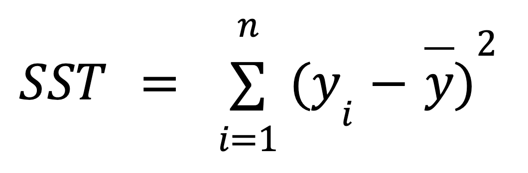
where:
The following plot for a simple linear regression demonstrates the meaning of the above formula graphically:
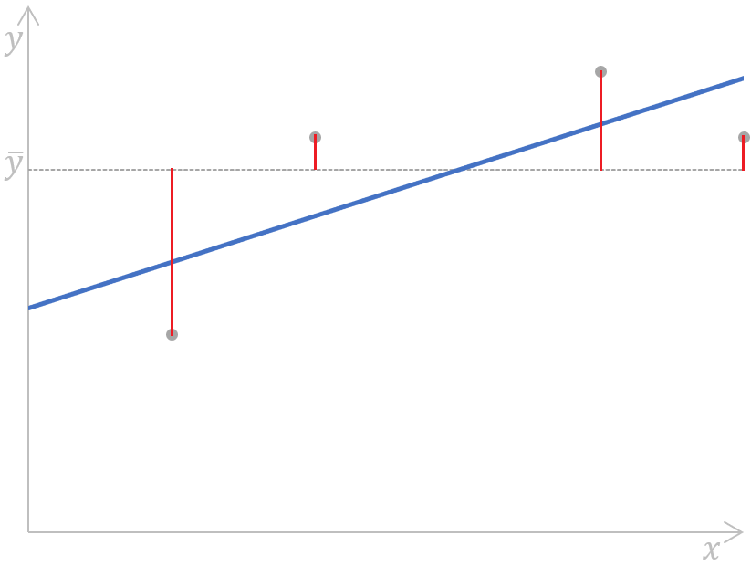
Calculating the sum of squares total for a simple linear regression. Image by Author
As we can see, the distances (the red segments on the plot) between the mean value (the grey dashed line) of the observed dependent variable and each value (the grey dots) of that variable are measured, squared, and summed up. In addition, this plot clearly shows that the SST doesn't depend on the regression model; it only depends on the observed y-values and the mean of the observed dependent variable.
The sum of squares regression (SSR) is the sum of squared differences between each value of the dependent variable predicted by a regression model for each data point of the independent variable and the mean of the observed dependent variable. Other terms for this metric include: regression sum of squares, sum of squares due to regression, and explained sum of squares. There’s even another abbreviation for it—ESS.
The sum of squares regression captures the portion of the total variability in the dependent variable explained by the regression model (hence one of its alternative terms—explained sum of squares). We can also think of it as the error reduced due to the regression model.
To calculate the SSR, we use the following formula:
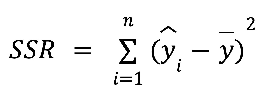
where:
We can illustrate this formula on the following simple linear regression plot:
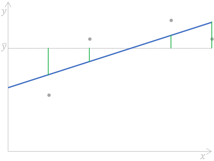 Calculating the sum of squares regression for a simple linear regression. Image by Author
Put simply, the distances (the green segments on the plot) between the mean value (the grey dashed line) of the observed dependent variable and each value of the dependent variable predicted by a regression model (the blue line) for each data point of the independent variable are measured, squared, and summed up.
In regression analysis, the SSR contributes to measuring the fit of a regression model by helping to determine how well the model predicts data points. We'll have a clearer picture of how it happens later on in this tutorial when we discuss the relationship between the three metrics of the sum of squares.
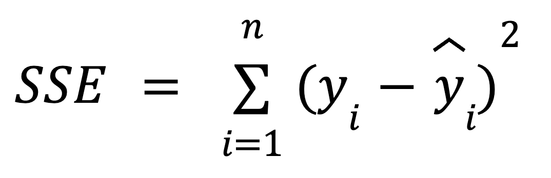
The sum of squares error (SSE) is the sum of squared differences between each value of the observed dependent variable and the value of the dependent variable predicted by a regression model for the same data point of the independent variable. In other words, this metric measures the difference between actual and predicted values of the dependent variable.
The sum of squares error is also called the error sum of squares, residual sum of squares, sum of squares residual, or unexplained sum of squares. Besides SSE, it can also be abbreviated as RSS, ESS, or even SSR—in the last case, it can be easily confused with the earlier discussed SSR which stands for the sum of squares regression.
The sum of squares error reflects the remaining error, or unexplained variability, which is the portion of the total variability in the dependent variable that can't be explained by the regression model (that's why it's also called the unexplained sum of squares).
We can use the following formula to calculate the SSE:
where:
Graphically, this formula can be displayed as:
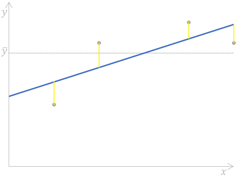 Calculating the sum of squares error for a simple linear regression. Image by Author
Here, the distances (the yellow segments on the plot) for each pair of actual-predicted values of the dependent variable are measured, squared, and summed up.
In regression analysis, minimizing the SSE is key to improving the accuracy of the regression model, and we're going to build intuition around it in the next chapter.
We also have a collection of technology-specific tutorials to help you gain the skills needed to build simple linear and logistic regression models, including Essentials of Linear Regression in Python, How to Do Linear Regression in R, and Linear Regression in Excel: A Comprehensive Guide For Beginners.
The mathematical relationship between the SST, SSR, and SSE is expressed by the following formula:

Earlier, we mentioned that the total variability (SST) is composed of both the explained variability (SSR) and the unexplained variability (SSE), which is reflected in the above formula.
As we saw earlier, the SST doesn’t depend on the regression model, while the other two metrics do. This means that improving the model's accuracy is related to changes in the SSR or SSE—in particular, by minimizing the SSE and, therefore, maximizing the SSR. From the above formula, we can say that the smaller the SSE, the closer the SSR to the SST; hence, the better our regression model fits the observed values of the dependent variable.
If the SSE were equal to 0, the SSR would coincide with the SST, which would mean that all the observed values of the dependent variable are perfectly explained by the regression model, i.e., all of them would be located exactly on the regression line. In real-world scenarios, this won’t happen, but we should aim to minimize the SSE to have a more reliable regression model.
Since the SST represents the total variability in the data, when we fit a regression model, we decompose this total variability into two parts: SSR and SSE. This decomposition is geometrically interesting because it reflects Pythagoras’ theorem in a high-dimensional space. This is because the total variability is partitioned into two orthogonal components: the variability explained by the model and the unexplained error. This interpretation makes sense because regression is essentially about projecting data onto a lower-dimensional space, which is the space spanned by our predictors. Take our Linear Algebra for Data Science in R to learn more about concepts like subspaces.
In ridge and lasso regression, the decomposition of SST into SSR and SSE does’t follow the same relationship. This is because both ridge and lasso add regularization terms, or penalties, to their respective cost functions, which alters the relationship. In the case of regularized versions of regression, the SST is still well-defined, but the explained variability and residual variability no longer sum up to SST because of the regularization term. Read our Regularization in R Tutorial: Ridge, Lasso and Elastic Net to learn more.
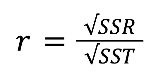
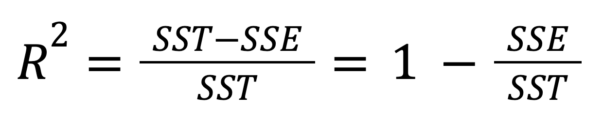
The R-squared, also known as the coefficient of determination, is an important statistical measure for evaluating the fit quality of a regression model and, hence, its predictive power. It represents the proportion of the variability in the dependent variable that can be explained by the independent variable. The R-squared can be calculated by squaring the correlation coefficient r, and it can also be calculated according to this formula:
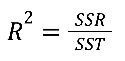
Or, alternatively:
Considering the relationship between the SST, SSR, and SSE, the above formula can be rewritten as:
The value of the R-squared can be from 0 to 1, inclusive. If R2 = 0, it means that our regression model doesn't explain any portion of the variability in the dependent variable at all. Instead, if R2 = 1, it means that our regression model perfectly explains the entire variability in the dependent variable. In practice, it's almost impossible to encounter these extreme values—most probably, in real-world cases, we'll see something in between.
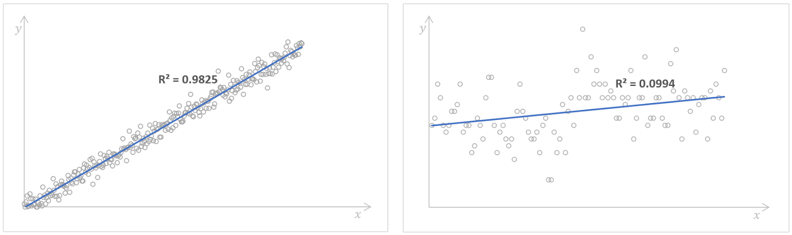
Regression models with high (left) and low (right) values of the R-squared. Source: Kaggle Number of Books Read and Kaggle Possum Regression. Image by Author.
A high value of the R-squared indicates good model performance, meaning that the dependent variable can be predicted by the independent variable with a high accuracy. However, there is no rule of thumb for which value of the R-squared should be considered as good enough. It depends on each particular case, the requirements for the precision of a regression model, and how much variability we expect to see in the data. Often, it also depends on the domain to which our regression analysis is related. For example, in scientific fields, we would seek for the value of the R-squared higher than 0.8, while in social sciences, the value of 0.3 could be already good enough.
As a final note, we should say that in multiple linear regression, meaning regression with more than one independent variable, we often consider the adjusted R-squared instead, which is an extension on the R-squared that accounts for the number of predictors and sample size.
While nowadays we can easily and quickly calculate the SST, SSR, and SSE in the majority of statistical software and programming languages, it's still worthwhile to really understand what they mean, their interconnection, and, in particular, their significance in regression analysis. The comprehension of the relationship between the three components of the variability and the R-squared helps data analysts and data scientists improve model performance by minimizing the SSE while maximizing the SSR, so they can make informed decisions about their regression models.
To build a strong foundation in statistics and learn powerful statistical techniques by working with real-world data, consider the following exhaustive and beginner-friendly skill tracks: Statistics Fundamentals in Python and Statistics Fundamentals in R. Lastly, if you are interested in how the regression coefficients are calculated, check out our Normal Equation for Linear Regression Tutorial and QR Decomposition in Machine Learning: A Detailed Guide.
Learn with DataCamp
Cours
Cours
Cours
Tutoriel
Josef Waples
Tutoriel
Allan Ouko
Tutoriel
Allan Ouko
Tutoriel
Allan Ouko
Tutoriel
Eladio Montero Porras
Tutoriel
Zoumana Keita