Benchmarking High-Performance pandas Alternatives

Introduction

Pandas is an extraordinarily powerful tool in Python's data science ecosystem, offering several data manipulation and cleaning capabilities. However, while great for medium-sized datasets, it can face performance issues when dealing with large datasets, prompting the need for high-performance alternatives.

This comprehensive article introduces some of these alternatives and compares them through benchmarking in terms of data loading time, execution time, memory usage, scalability, and ease of use.

Note: Benchmarking results vary a lot depending on your hardware setup.

Understanding the Benchmarks

Benchmarks are a point of reference against which software or hardware may be compared for performance evaluation. This reference is relevant in software performance optimization as it allows us to measure the efficiency of different methods, algorithms, or tools. In this context, the key metrics for benchmarking data manipulation libraries include execution time, memory usage, scalability, and ease of use.

Introduction to High-Performance Alternatives

The main alternative Python tools are Polars, Vaex, and Datatable. Before diving into their comparative analysis, let’s have a quick overview of what each one of these tools is.

Polars

Polars can be described by three key features. First, it offers a comprehensive Python API filled with numerous functions to handle Dataframes. Second, it can serve dual purposes - it can be employed as a library for Dataframes or as the underlying query engine for data models. Lastly, by incorporating the secure Arrow2 implementation of the Apache Arrow specification, Polars becomes a highly efficient tool for processing large amounts of data.

You can check out our introduction to Polars tutorial, as well as a comparison between pandas 2.0 and Polars.

Vaex

Vaex is for lazy, out-of-core DataFrames (similar to Pandas) to visualize and explore big tabular datasets. It can be very efficient as it delays operations until necessary (lazy evaluation), reducing memory usage and time.

Datatable

Datatable can be used for performing large data processing (up to 100GB) on a single-node machine at the maximum speed possible. One of the important features of Datatable is its interoperability with Pandas/NumPy/pure Python, which allows users to easily convert to another data-processing framework.

To learn more about pandas, our pandas Tutorial Dataframes in Python is a great starting point.

Also, the pandas Cheat Sheet for Data Science in Python gives a quick guide to the basics of the Python data analysis library, along with code samples.

Setting up the Benchmarking Environment

This section covers the creation of the benchmarking data and the installation of all the libraries involved in the benchmarking analysis.

Benchmarking data

The benchmarking data set is 5.7 GB large, which is large enough to perform a decent comparison. Each row has been duplicated 100000 times, resulting in 76 800 000 rows. Diabetes data is the original one being used and is freely available from Kaggle.

The final benchmarking notebook is available on GitHub.

import pandas as pd

data_URL = "https://raw.githubusercontent.com/keitazoumana/Experimentation-Data/main/diabetes.csv"

original_data = pd.read_csv(data_URL)

# Duplicate each row 100000 times
benchmarking_df = original_data.loc[original_data.index.repeat(100000)]

# Save the result as a CSV file for future use.
file_name = "benchmarking_data.csv"

benchmarking_df.to_csv(file_name, index=False)

Installation of the libraries

Now, we can proceed with the installation of all the libraries involved in the benchmarking analysis.

From a Jupyter notebook environment, all the installation is performed from the pip install command as follows:

%%bash
pip3 -q install -U polars
pip3 -q install vaex
pip -q install datatable

After successfully running the above code block, we can import them with the import statement:

import pandas as pd
from time import time
import polars as pl
import vaex as vx
import datatable as dt

Furthermore, we use the plotly library for visualization purpose.

import plotly.express as px

Now we are all set to proceed with the benchmarking analysis.

Benchmarking Execution Time

The execution time will be evaluated for the following operations: data loading, data offloading, data aggregation, and data filtering. A helper function is implemented for each task and will return a dictionary with two main keys: the library name and the execution time.

The plot metrics function is then used to plot the result in a graphical manner using the Plotly Express library. It has two parameters: the list of all the dictionaries from the previous helper functions and the title of the underlying graphic.

def plot_metrics(list_exec_time, graph_title):

	df = pd.DataFrame(list_exec_time)

	fig = px.bar(df, x='library', y= 'execution_time', title=graph_title)
    
	fig.show()

Data loading

The helper function read_csv_with_time has two main parameters: the file name to be read and the library name.

def read_csv_with_time(library_name, file_name):

	final_time = 0

	start_time = time.time()

	if library_name.lower() == 'polars':
    	df = pl.read_csv(file_name)

	elif library_name.lower() == 'pandas':
    	df = pd.read_csv(file_name)

	elif library_name.lower() == 'vaex':
    	df = vx.read_csv(file_name)

	elif library_name.lower() == 'datatable':
    	df = dt.fread(file_name)

	else:
    	raise ValueError("Invalid library name. Must be 'polars', 'pandas', 'vaex', or 'datatable'")

	end_time = time.time()

	final_time = end_time - start_time

	return {"library": library_name, "execution_time": final_time}

The function can be applied using each of the libraries, starting with pandas.

pandas_time, pandas_df = read_csv_with_time('pandas', file_name)
polars_time, polars_df = read_csv_with_time('polars', file_name)
vaex_time, vaex_df = read_csv_with_time('vaex', file_name)
datatable_time, dt_df = read_csv_with_time('datatable', file_name)

The resulting dictionaries can be combined as a list and plotted using the following expression.

exec_times = [pandas_time, polars_time,
           vaex_time, datatable_time]

def plot_metrics(list_exec_time, graph_title):

 [print(exec_time) for exec_time in list_exec_time]
 df = pd.DataFrame(exec_times)

 # Plot bar plot using Plotly Express
 fig = px.bar(df, x='library', y='execution_time', title=graph_title)
 fig.show()

plot_metrics(exec_times, "Read Execution Time Comparison")

{'library': 'pandas', 'execution_time': 35.07908916473389}
{'library': 'polars', 'execution_time': 6.041005373001099}
{'library': 'vaex', 'execution_time': 36.431522607803345}
{'library': 'datatable', 'execution_time': 4.4584901332855225}

Dictionary format of the execution times for data loading

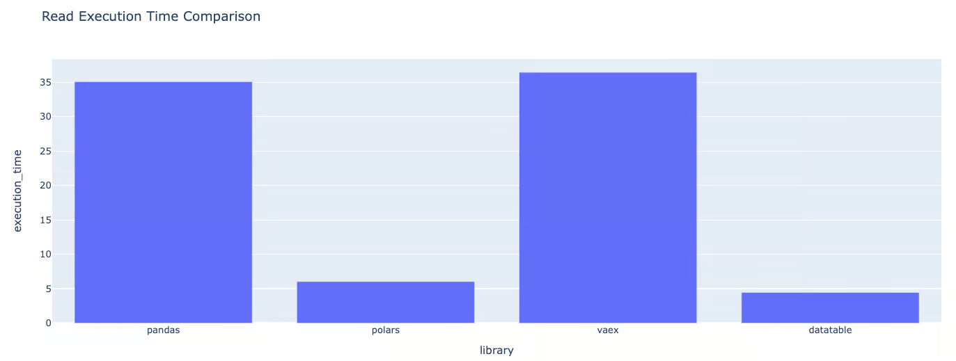
Graphic format of the execution times for data loading

Based on the graphics, we can conclude that Polars is:

• Polars is 1.35 times slower than Datatable
• Pandas is 7.87 times slower than DataTable.
• Vaex is approximately 8.17 times slower than DataTable.

Data grouping

Similarly, the group_data_with_time is responsible for tracking the execution time for grouping the column provided in parameter. In this case, we are using the Pregnancies column.

from time import time

def group_data_with_time(library_name, df, column_name='Pregnancies'):

 start_time = time()

 if library_name.lower() == 'polars':
     df_grouped = df.group_by(column_name).first()

 elif library_name.lower() == 'vaex':
     df_grouped = df.groupby(column_name, agg='first')

 elif library_name.lower() == 'pandas':
     df_grouped = df.groupby(column_name).first()

 elif library_name.lower() == 'datatable':
     df_grouped = df[:, dt.first(dt.f[:]), dt.by(column_name)]

 else:
     raise ValueError("Invalid library name. Must be 'polars', 'vaex', or 'datatable'")

 end_time = time()

 final_time = end_time - start_time

 return {"library": library_name, "execution_time": final_time}

pandas_time = group_data_with_time('pandas', pandas_df)
polars_time = group_data_with_time('polars', polars_df)
vaex_time = group_data_with_time('vaex', vaex_df)
datatable_time = group_data_with_time('datatable', dt_df)

exec_times = [pandas_time, polars_time,
           vaex_time, datatable_time]
plot_metrics(exec_times, "Grouping Execution Time Comparison")

{'library': 'pandas', 'execution_time': 2.382519245147705}
{'library': 'pandas', 'execution_time'': 1.0898876190185547}
{'library': 'pandas', 'execution_time': 0.8506548404693604}
{'library': 'pandas', 'execution_time': 0.34698963165283203}

Graphic format of the execution times for data grouping

For the updated data grouping task, comparing the fastest library DataTable to the others:

We can see that DataTable is the fastest among the evaluated libraries.

• Vaex is 2.45 times slower than DataTable.
• Polars is 3.14 times slower than DataTable.
• Pandas is 6.87 times slower than DataTable.

This analysis demonstrates DataTable's superior efficiency for data grouping tasks, with Vaex being relatively close in performance. Polars and Pandas exhibit similar execution times, both significantly slower than DataTable.

Column Sorting

Using the same approach, the column sorting function sorts the given column using each library.

def sort_data_with_time(library_name, df, column_name='Pregnancies'):
    
	start_time = time()

	if library_name.lower() == 'polars':
    	df_sorted = df.sort(column_name)
	elif library_name.lower() == 'vaex':
    	df_sorted = df.sort(column_name)

	elif library_name.lower() == 'datatable':
    	df_sorted = df.sort(column_name)
   	 
	elif library_name.lower() == 'pandas':
    	df_sorted = pd.DataFrame(df).sort_values(column_name)
	else:
    	raise ValueError("Invalid library name. Must be 'polars', 'vaex', 'datatable', or 'pandas'")

	end_time = time()

	final_time = end_time - start_time

	return {"library": library_name, "execution_time": final_time}

pandas_time = sort_data_with_time('pandas', pandas_df)
polars_time = sort_data_with_time('polars', polars_df)
vaex_time = sort_data_with_time('vaex', vaex_df)
datatable_time = sort_data_with_time('datatable', dt_df)

{'library': 'pandas', 'execution_time': 6.735127687454224}
{'library': 'polars', 'execution_time': 4.119458436965942}
{'library': 'vaex', 'execution_time': 1.0371737480163574}
{'library': 'datatable', 'execution_time': 0.3971593379974365}

Dictionary format of the execution times for data sorting

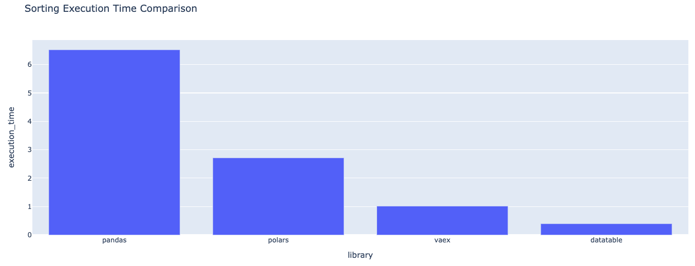
Graphic format of the execution times for data sorting

For the data sorting task, DataTable is the fastest among the evaluated libraries.

• Vaex is 2.61 times slower than DataTable.
• Polars is 10.37 times slower than DataTable.
• Pandas is 16.96 times slower than DataTable.

This analysis shows DataTable's superior performance in handling data sorting tasks, significantly outpacing Vaex, Polars, and Pandas, with Vaex being the closest in performance but still more than twice as slow.

Data Offloading

With data offloading, the idea is to convert the original data into a different format, which numpy array in this specific scenario.

def offload_data_with_time(library_name, df):
    
	start_time = time()

	if library_name.lower() == 'polars':
    	array = df.to_numpy()
   	 
	elif library_name.lower() == 'vaex':
    	array = df.to_pandas_df().values

	elif library_name.lower() == 'datatable':
    	array = df.to_numpy()
   	 
	elif library_name.lower() == 'pandas':
    	array = pd.DataFrame(df).values
	else:
    	raise ValueError("Invalid library name. Must be 'polars', 'vaex', 'datatable', or 'pandas'")

	end_time = time()

	final_time = end_time - start_time

	return {"library": library_name, "execution_time": final_time}

exec_times = [pandas_time, polars_time,
           vaex_time, datatable_time]

plot_metrics(exec_times, "Data offloading Execution Time Comparison")

{'library': 'pandas', 'execution_time': 1.8406445980072021}
{'library': 'polars', 'execution_time': 3.238591432571411}
{'library': 'vaex', 'execution_time': 6.945307970046997}
{'library': 'datatable', 'execution_time': 2.634136438369751}

Dictionary format of the execution times for data offloading

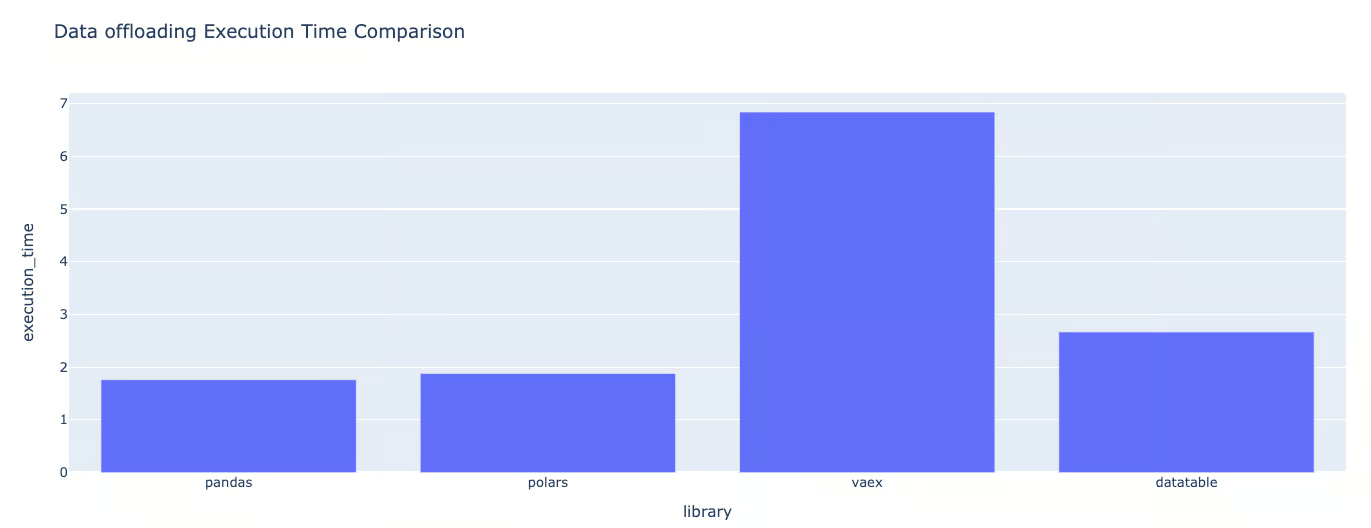
Graphic format of the execution times for data offloading

Data offloading is the last round of the benchmarking for the execution time.

This time, Vaex is the one with the highest execution time. Comparing pandas to these libraries, we can see that its execution time is approximately:

• DataTable is 1.43 times slower than Pandas.
• Polars is 1.76 times slower than Pandas.
• Vaex is 3.77 times slower than Pandas.

Benchmarking Memory Usage

The execution time is not the only criterion when comparing different libraries. Knowing how efficiently they deal with memories is also important to consider. This section shows two different memory usage using the tracemalloc library:

• Current memory usage. The total amount of memory used during the execution using a specific library. It corresponds to the RAM space being occupied at that time.
• Peak memory usage. Corresponds to the maximum amount of memory used by the program. It is important to know that the peak memory is always higher than the current memory.

Having these visualizations helps understand which program uses as much memory, leading to out-of-memory errors, especially when working with large datasets.

In addition to tracemalloc, the os library is also required.

import tracemalloc as tm
import os

Before starting, we create an empty list that will hold the result of each memory usage value.

list_memory_usage = []

For each library, the estimation of the memory usage is done with the general syntax below corresponding to the execution with the Vaex library. Also, this focuses only on the memory usage for the data offloading tasks.

tm.start()
vaex_time = offload_data_with_time('vaex', vaex_df)
memory_usage = tm.get_traced_memory()
tm.stop()

list_memory_usage.append({
	'library': 'vaex',
	'memory_usage': memory_usage
})

The syntax is the same for the remaining libraries, and we get the following instructions, respectively for Polars, pandas, and Datatable:

tm.start()
polars_time = offload_data_with_time('polars', polars_df)
memory_usage = tm.get_traced_memory()

tm.stop()

list_memory_usage.append({
	'library': 'polars',
	'memory_usage': memory_usage
})

tm.start()
offload_data_with_time('pandas', pandas_df)

# Get the memory usage
memory_usage = tm.get_traced_memory()

tm.stop()

list_memory_usage.append({
	'library': 'pandas',
	'memory_usage': memory_usage
})

tm.start()
datatable_time = offload_data_with_time('datatable', datatable_df)
memory_usage = tm.get_traced_memory()

tm.stop()

list_memory_usage.append({
	'library': 'datatable',
	'memory_usage': memory_usage
})

After the execution of all the previous code, we can plot the graphic using the helper function below:

def plot_memory_usage(list_memory_usage, graph_title='Memory Usage by Library'):

	df = pd.DataFrame(list_memory_usage)

	# separate the memory usage tuple into two columns: current_memory and peak_memory
	df[['current_memory', 'peak_memory']] = pd.DataFrame(df['memory_usage'].tolist(), index=df.index)

	# now we no longer need the memory_usage column
	df = df.drop(columns='memory_usage')

	# melt the DataFrame to make it suitable for grouped bar chart
	df_melted = df.melt(id_vars='library', var_name='memory_type', value_name='memory')

	# create the grouped bar chart
	fig = px.bar(df_melted, x='library', y='memory', color='memory_type', barmode='group',
             	labels={'memory':'Memory Usage (bytes)', 'library':'Library', 'memory_type':'Memory Type'},
             	title=graph_title)
    
	fig.update_layout(yaxis_type="log")
	fig.show()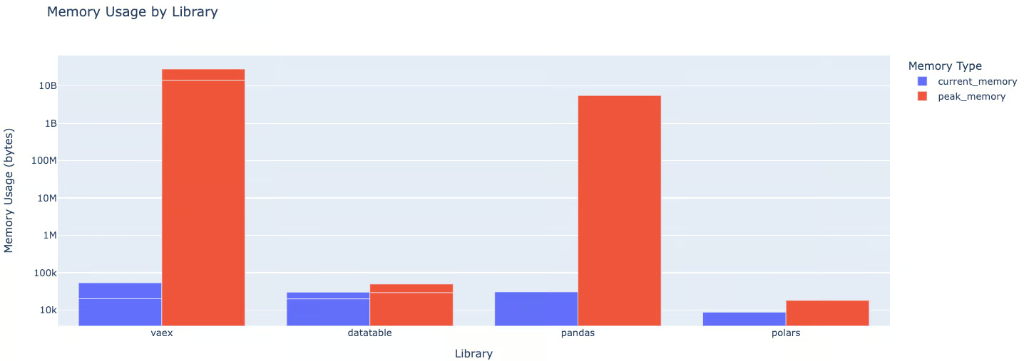

We can notice that:

• Pandas uses approximately 1100 times more current memory than Polars, 7.4 times more than Vaex, and 29.4 times more than Datatable.
• When it comes to peak memory usage, both pandas and Vaex use around 963K times more memory than Polars and 131K times more than Datatable.

Further analysis, such as Dask vs pandas speed, could provide a broader overview.

Pandas Alternatives Comparison Table

Below, we’ve compiled our findings into a comparison table, showing the differences between Polars, Vaex, and Datatables:

Conclusion

Different factors must be considered when performing the scalability and ease of integration analysis. Our benchmarking highlighted that even though pandas is well-established and user-friendly and has a steeper learning curve, it does not efficiently handle large datasets.

However, there are different ways that be adapted on how to speed up pandas, and our High-Performance Data Manipulation in Python: Pandas 2.0 vs Polars can help with that.

Vaex performance varies depending on the task. So, choosing an alternative to Pandas depends on the users’ specific demands, dataset sizes, and their ability to handle the learning curve and integration.