Data Wrangling with INDEX-MATCH in Spreadsheets

Usually, when one is taught to use Excel for the first time, chances are that VLOOKUP will be introduced as the primary method for data wrangling. VLOOKUP is indeed a powerful function that can handle many tasks related to data handling as illustrated in Data Wrangling with VLOOKUP in Spreadsheets. In the same tutorial, we also covered the basics of the INDEX-MATCH combination, which is another method to perform vertical table lookups that has several advantages over VLOOKUP at the cost of a more complicated formula.

These advantages include features such as:

• Dynamic Column References: These allow you to insert and delete columns safely from your dataset without affecting the lookup function.
• Higher Processing Speeds in Large Datasets: If your tables are extensive, you will likely notice that INDEX-MATCH is much faster than VLOOKUP due to INDEX-MATCH caring about the column you want to retrieve and the lookup column only.
• Location of the Lookup Values: VLOOKUP cannot look at any value located to the left of the first column you select in the table range, but INDEX-MATCH can look horizontally too, so it doesn't have that limitation.
• Limited Lookup Value Size: VLOOKUP cannot look up values longer than 255 characters, but INDEX-MATCH can.

Furthermore, INDEX-MATCH also allows matching based on the value of multiple columns, and case-sensitive matching, which is very useful when you have to deal with certain IDs that may differ based on lower and upper case letters. That is why this tutorial will aim to dive deeper into the advanced features of the INDEX-MATCH combination, as well as, show examples of how these features can come in handy.

The Basics of INDEX-MATCH

In its most simple form, INDEX-MATCH can be used in the same way as VLOOKUP, to perform simple vertical table lookups based on a common key. The basic structure of the formula can be seen as follows:

=INDEX(column_range, MATCH(lookup_value, lookup_column_range, match_type))

• column_range: The range of the column whose value you want to retrieve.
• lookup_value: The value you want to look up (the key).
• lookup_column_range: The range of the column that contains the keys that you want to match.
• match_type: Either a 0 or a 1. With 0 indicating an exact match and 1 indicating an approximate match. It is analogous to the FALSE/TRUE flag in VLOOKUP.

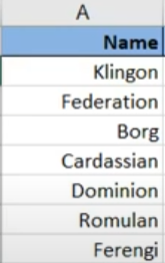
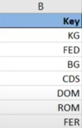
Next, let's illustrate how INDEX-MATCH works using a couple of toy tables. This first table contains some names, as well as some unique keys. The second table contains the same keys (though not necessarily in the same order) and some descriptions. Thus, the task is to join the descriptions in the second table with the names in the first table using INDEX-MATCH. The tables can be seen below:

As you can see, the first table is lacking the description. Lets now proceed to join the name with its description using INDEX-MATCH:

Easy right? As you can see in the video, the first step is to select a column_range that contains the data that we want to retrieve inside the INDEX function. In this case, that is the Description (M2:M8). The second step is to select the lookup_value inside the MATCH function, that is, cell B2. Lastly, we add the lookup_column_range (L2:L8) inside the MATCH function, and we select 0 as the match_type since we want an exact match of the lookup_value. The rest is just hitting ENTER and dragging down the formula to finally join the name with the descriptions.

INDEX-MATCH can also be used to join tables that are on separate sheets like in VLOOKUP. An example video can be seen below:

Note: You may have noticed that the column ranges that I select in the videos tend to be surrounded by $ signs. This is done in order to select fixed ranges that are not altered when you drag the formulas vertically or horizontally. I will keep using that notation across this tutorial.

So far all this behaves very much like a simple VLOOKUP but with a bit more hassle. Nevertheless, as mentioned at the beginning of this tutorial, there are various advantages if you take the INDEX-MATCH route. One of the most useful is dynamic column references. That is, allowing you to add columns to the table range where you are looking up values without affecting the lookup itself.

If we added a new column in our toy example and we were using VLOOKUP, we would have to rewrite the formula in the left table to reference the description, which would become column 3. However, if you use INDEX-MATCH, which has dynamic column references, this is not needed. This comparison can be seen in the video below:

The example above illustrates how the column that was performing the lookup using INDEX-MATCH adjusted when the new column containing the space ship types was added, while the column that had VLOOKUP did not. This advantage of INDEX-MATCH over VLOOKUP really shines in tasks involving lookups in large Excel tables such as a business sales report. In other words, imagine you have several business dashboards built in Excel and that all reference a single table with all the data. If you are using VLOOKUP and one day it becomes necessary to insert a column in the middle to add another feature, you would have to change the VLOOKUP function calls in all the dashboards that depend on that table. However, if you built the dashboards using INDEX-MATCH as your lookup method, you will not have to face such an issue.

Advanced INDEX-MATCH: Case Sensitive Matching

Dynamic column references are very useful, but that is not all the advantages that INDEX-MATCH has to offer. For example, it is possible to enhance the basic syntax of INDEX-MATCH to perform case sensitive lookups. In particular, we are going to add an EXACT function inside the MATCH function to accomplish this. The detailed syntax can be seen below:

{=INDEX(data_range, MATCH(TRUE,EXACT(lookup_value, lookup_column_range), match_type), desired_column_number)}

• data_range: The table range of interest that includes the lookup column and the desired column that you want to retrieve.
• lookup_value: The value you want to look up (the key)
• lookup_column_range: The range of the column that contains the keys that you want to match
• match_type: Either a 0 or a 1. With 0 indicating an exact match and 1 indicating an approximate match. It is analogous to the FALSE/TRUE flag in VLOOKUP
• desired_column_number: Same as the column index number in VLOOKUP. This is the column index that contains the data that you want to obtain.

Case sensitive matching using this modified INDEX-MATCH combination can be very useful when matching keys that contain letters and that are differentiated by the case of these letters (a.k.a say you have two different keys one is "00567UUp" and the other is "00567UUP"). These situations can be encountered, for example, inside the widely used Salesforce CRM when trying to match Account IDs or Sales Opportunities IDs. For now though, we won't be using any Salesforce datasets, but we will be using a modified version of our toy tables in the video below to illustrate how the above formula works in action.

Note: that the function combination above is enclosed in curly braces. This means that this is an array formula and must be entered pressing Cntr+Shift+Enter.

As you can see the syntax of this formula can be long to write, but the results are just as you would expect. It looks up the values just like the normal INDEX-MATCH, but taking into account the case of the characters. The magic here is done by the EXACT function that returns an array of TRUE and FALSE. Wherever it is TRUE in this array, you can say that there is a value that has the same exact case. After that, the MATCH function takes care of gathering the position of the first TRUE occurrence.

Please note that it is crucial that you hit Cntrl+Shift+Enter when you finalize writing the formula or you will get an #N/A error that can be hard to diagnose.

Advanced INDEX-MATCH: Matching Based on Multiple Features

Case sensitive lookups in Excel is quite cool, but there is one feature that is even better; lookups that take into account multiple criteria. Taking into account numerous criteria is something that it is commonly done as part of conditional count or sum functions like COUNTIFS or SUMIFS, but it is more exotic to see it as part of lookup functions in Excel. Nevertheless, it can be advantageous in certain situations. For instance, it could be the way to if, say, you have an HR Excel file, and you want to look up the salary of a given employee based on its first AND last names. If you take into account only one of the two columns, it is possible that you get the salary of the wrong Employee since there can be many with the same first name or last name. However, it is much more likely to get the correct person if you retrieve the value based on both first and last names.

With that said, let us now look at the structure of INDEX-MATCH taking into account multiple features:

{=INDEX(column_range, MATCH(1,(lookup_value_1 = lookup_column_range_1)*(lookup_value_2 = lookup_column_range_2)*...(lookup_value_n = lookup_column_range_n), match_type))}

For the most part, the formula has the same exact components as the normal INDEX-MATCH, but it can now take into account $n$ lookup values with its respective number of lookup ranges. If you need a refresher of what these components are, you can scroll up to the basic INDEX-MATCH syntax. The reason why we have a "1" in the MATCH function is that this formula creates arrays of 1s and 0s that represent the matches of each of the desired criteria. It then uses the MATCH function to retrieve the location of the first 1 that is found.

As with the case sensitive formula, this one is also covered in curly braces, which means that you must hit Cntr+Shift+Enter when you finish writing it as this is an array formula.

Let us look at an example of how this formula works in action by trying to select spaceships that belong to a given race and that have a given maximum warp speed in the video below:

Voilá! Now you have the tools to match arguments based on multiple keys. Keep in mind that in this small toy example, I have only used two, the key and the max warp speed, but in theory, you could keep adding criteria if you wish so. To get back to our HR example, you could match based on first and last names as well as job title to minimize the chance of getting the wrong employee's salary.

Conclusion

Congratulations! You are now familiar with INDEX-MATCH and the variety of things that you can accomplish with it beyond a simple vertical lookup. If at some point you are tasked with taking care of complex Excel reports, this function combination will likely become your best friend. Like many, I was taught VLOOKUP in school, but when I seriously started using Excel for tasks such as the case sensitive lookups of Salesforce account IDs, I realized that INDEX-MATCH was a much better option in the long run, despite the hassle and error-prone that can be to write the formula. I encourage you to try it out next time you have to do a vertical lookup in your Excel endeavors. Who knows, maybe you will take a liking to it as I did.

If you feel like learning even more, feel free to take a look at DataCamp's Data Analysis with Spreadsheets Course.