Data Wrangling with VLOOKUP in Spreadsheets

Sometimes, data science is not about deep learning, big data or recommendation systems. At times, particularly if you are employed in a sector like finance or a company that has relied heavily on Excel in the past, chances are that you will have to deal with Excel spreadsheets a lot. I confess myself to belong to the latter example. My employer relied heavily on Excel and, as such, I had to learn a lot about its various capabilities for some of my work responsibilities.

Even though R and Python have apparent advantages over Excel in many ways, Excel is still a powerful tool for certain tasks like creating business reports. For this tutorial though, I am going to be focusing on one of Excel's built-in functions that greatly helps when working with various Excel tables at the same time.

The function I am referring to is VLOOKUP. VLOOKUP allows the user to relate different columns in the same sheet or between different sheets in the same workbook. In essence, it will enable the user to look up a value from one column and returns its corresponding value from a different column. This functionality becomes very useful if you have large data tables that are not sorted and you need to relate them based on some column (ideally containing a unique key).

Let me illustrate how the process of using the VLOOKUP function works between columns in the same sheet with a toy data table:

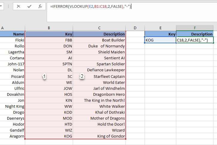
What you can see in the screenshot above is a common VLOOKUP expression written as you would for a business report. Its components are as follows:

• IFERROR function: Used to substitute an error with a hyphen (-) if the key was empty or if it was not present in the data table. It is just a good practice for error handling that makes the sheet cleaner when an error occurs, but it's certainly not needed to make VLOOKUP work.
• VLOOKUP arguments:
  • E2 is the lookup value (in this case we used KOG as an example, but it could be any of the keys). This value has to be located in the leftmost column of the selected table range that you want to search.
  • B1:C18 is the table range/array to look values. The leftmost column has index 1 as shown. This column must also be the one containing the lookup values for the function to work.
  • 2 is the column index number of the selected table range that you want to retrieve the value from. In this example we want to retrieve the description so we pick column 2 of the table array.
  • FALSE is a flag to indicate that you want an exact match of the lookup value. In this case, we picked FALSE since you want an exact match of KOG key. The other option is to select TRUE, which seeks an approximate match of the lookup value and it is default if you don't specify this argument. You generally would not advise to select TRUE if you are matching keys or strings since it can yield odd results.

Now, after writing that VLOOKUP statement, if you press ENTER in Excel, you will get the following result:

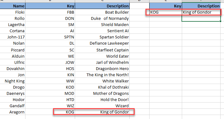
As you can see the VLOOKUP function returned just what you would expect "King of Gondor", which is the description associated with the KOG key. This is true for any key that you enter now in the cell E2. For instance, let's see what happens if we input the key KIN.

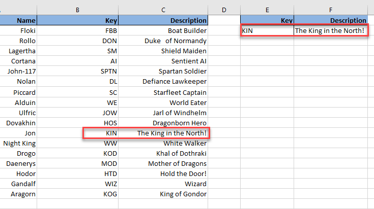
The King in the North! That's right if we enter the KIN key we would expect to get as it is the description for our dear Jon(Snow).

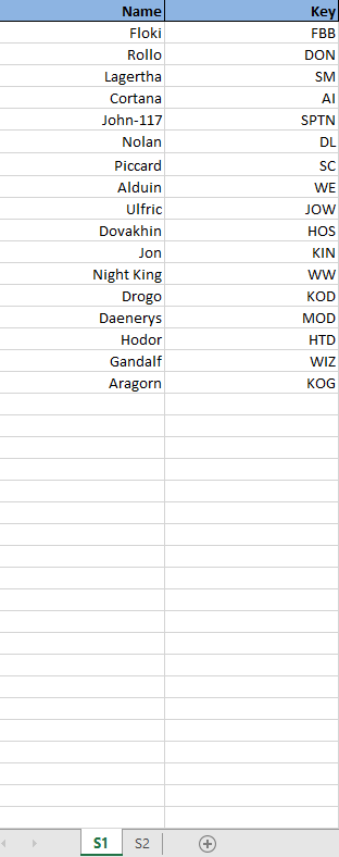
However, VLOOKUP has more uses than retrieving a single value depending on a key. Let's suppose for instance that we split that table into two each placed on a different sheet in the same workbook.

Joining Tables

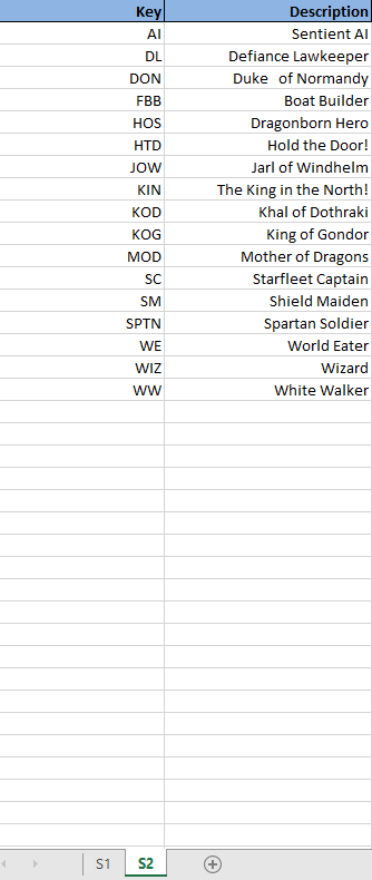As you can see, now the data is split into two different sheets (S1 and S2) and the keys on the table on the second sheet (S2) are in a different order. Lucky for us, the key column is common to both sheets regardless of the order so we can join the data together in S1 using VLOOKUP (you can think of it as a single-column left join). The syntax to achieve this is as follows:

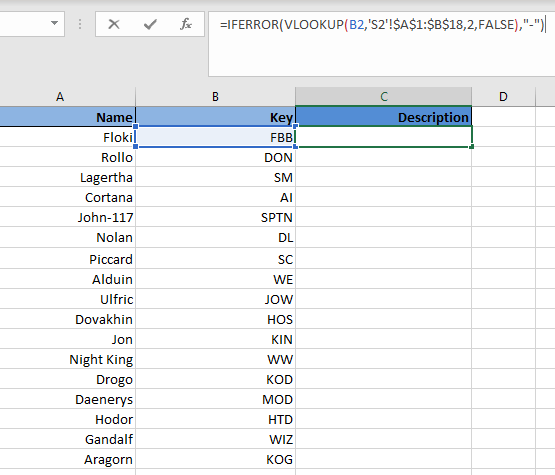
This time, the first argument, the lookup value, becomes B2 since we want to match the key B2 in the table on S2. The table range now becomes the entire data table in S2 with the first column containing the common keys. You may notice that the table range has dollar signs embedded. This is done by pressing F4 after obtaining the range, and it serves to lock the range down in such a way that, when you drag the formula down in S1, the VLOOKUP function will keep looking at the original range without moving it down as well. The column index number stays at 2 since we want the description, which is the second column in S2. Finally, the last argument we want is FALSE since we want an exact match for the keys.

The last step is to simply drag down the formula down to the last entry of the table. The resulting table in S1 is as follows:

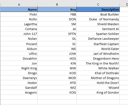
Voilá! Just like that, we stitched the data back together using VLOOKUP. Joining tables like this is a very common thing to do when working on a business setting and SQL, R or Python is not the tool that senior executives are used too. For example, you may have two files containing different details about qualified sales opportunities that can be related using a unique opportunity ID for a monthly sales Excel report (best example of Excel usage in my case).

Using Approximate Matches

So far you may have noticed that we have neglected using TRUE as the last argument (aka an approximate match) in any of my VLOOKUP functions. This is due to the fact that we have focused on exactly matching unique keys. However, you can use TRUE for the last argument in VLOOKUP safely when dealing with numerical data.

For instance, let's pretend we sell fish, and we offer the following discounts when customers by certain amounts (If anybody asks why fish, it's simple. Fish are awesome!).

The VLOOKUP function inside cell F2 this time is:

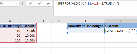
Once you have that formula in place, the discount will become the closest to the thresholds in the table. For instance, if we buy 25 fish our discount will be 5%, if we buy 70 fish, our discount will be 10%, and if we buy 120, then our discount will be 15%. All these examples can be seen below:

Introduction to INDEX-MATCH

VLOOKUP is a powerful function to relate different columns. However, there is an alternative way of doing this; the INDEX-MATCH combination. Unlike VLOOKUP that is a single function, INDEX-MATCH is a combination of two functions, and it has several advantages over the standard VLOOKUP even though it may be a bit more complex to write.

For the purposes of this tutorial, we will go over a simple example where we use INDEX-MATCH to join two tables based on a common key like we did above with VLOOKUP and explain the syntax (see below).

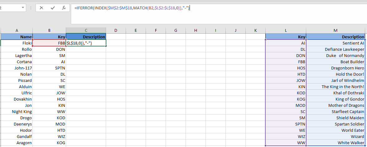
The components of the INDEX-MATCH combination are as follows:

• INDEX Arguments:
  • M2:M18: This is the column range whose values you want to retrieve, in this case, we want the description column, so we select that range. Note that we have used F4 after selecting the range to lock it down, so it doesn't move when we drag the formula.
• MATCH arguments:
  • B2: This is the key we want to look up. It is the equivalent of the lookup value in VLOOKUP.
  • L2:L18: This is the column range containing the keys where the lookup value has to be located. Note that we have also used F4 here.
  • 0: This is the same as FALSE in VLOOKUP. That is a flag for an exact match.

Looking at the syntax, one can already realize one of the main advantages of INDEX-MATCH over VLOOKUP. With INDEX-MATCH we have column immunity. That is, if now we decided to add an additional column between the Key and the Description in the right table above, it would not matter since the formula would adjust to reference the Description column still. You can see this below:

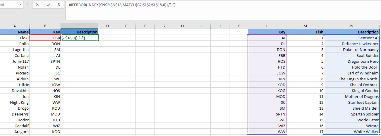
With VLOOKUP this is not possible without going back into the formula since it has a static column reference. In other words, in the example above, initially, you would have put a 2 as the column index number to retrieve the Description. However, after adding the Fish column, the VLOOKUP function would now return the value in the Fish column since that is now column 2 in the table range. You have to go to the VLOOKUP function manually and change the column index number to 3 for the function to work correctly again.

With that shown, to join the description to the name in the table on the left using INDEX-MATCH is the same procedure as with VLOOKUP. We simply drag the formula down as shown below:

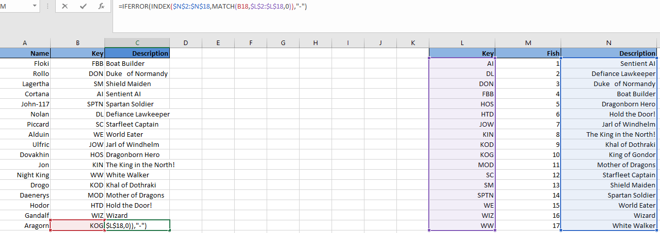
Note that for joining tables between different sheets in the same workbook is just the same procedure. The only difference is that you would have to select the column range containing the common keys as well as the column range whose values you want to retrieve from the second sheet.

Conclusion

I hope you have enjoyed the tutorial. These functions, VLOOKUP and INDEX-MATCH, are pretty much essential to anyone working with Excel on a business setting. I encourage you to dive deeper into INDEX-MATCH beyond what is covered here as it has many neat capabilities such as case sensitive matching (Yes, by default INDEX-MATCH and VLOOKUP are case insensitive) or matching based on multiple columns. Keep learning; the sky is the limit!

If you would like to learn more about VLOOKUP, take DataCamp's Data Analysis with Spreadsheets course.