How to Use HLOOKUP in Excel

Knowing enough about Microsoft Excel has become an essential skill for beginner data analysts due to its widespread use in the industry and its user-friendly interface.

Despite the realization of the need for complex data architectures and big data analytics tools to tackle the amount of big data collected, processed, and analyzed, many organizations still rely on Excel for data storage, manipulation, and analysis, making it one of the most commonly used tools for analytics purposes.

It’s rare not to see an organization using Microsoft Excel for a quick ad-hoc analysis on a snapshot of the data. Thus, data analysts must be equipped with Excel skills, especially built-in functions such as pivot tables, conditional formatting, lookup functions, and more.

After all, it’s quite easy to learn in a relatively short time without the need for advanced programming skills.

This tutorial will introduce you to one such built-in function — HLOOKUP. I’ll provide you with the syntax and help familiarize you with its usage with several examples. With multiple instances, including screenshots and frequently asked questions,   this tutorial will be everything you need to start using HLOOKUP in Excel.

What is HLOOKUP?

HLOOKUP (Horizontal Lookup) in Excel is a built-in function that enables users to find data in tables horizontally. It searches for a specific value in a table’s top row and returns a value from a row specified in the table or array.

HLOOKUP is useful in scenarios where you need to retrieve information from a data set that is arranged in rows rather than columns.

It is particularly handy when dealing with data tables where the key values are spread across the top row, and you need to extract corresponding values from lower rows based on a horizontal match.

The syntax and parameters for the HLOOKUP function

The syntax for HLOOKUP in Excel is as follows:

=HLOOKUP(lookup_value, table_array, row_index_num, [range_lookup])

The parameters of the function are:

• lookup_value: This is the value you want to search for in the first row of your table_array. It can be a value, a reference to a cell containing the value, or a text string.
• table_array: This is the range of cells that contains the data you want to search. The function will look for the lookup_value in the first row of this table_array.
• row_index_num: This is the row number in the table_array to retrieve the value. The first row of the table_array is considered row 1. This parameter specifies which row (from the top) in the table_array to return the value from, once the match is found in the first row.
• [range_lookup]: This optional parameter specifies whether you want HLOOKUP to find an exact or approximate match. If TRUE or omitted, HLOOKUP will use an approximate match. If this is the case, the values in the first row of table_array must be placed in ascending order. If FALSE, HLOOKUP will only find an exact match.

It’s important to note that if the [range_lookup] parameter is set to TRUE or omitted and an exact match is not found, the function will return the value corresponding to the largest value that is less than or equal to the lookup_value, assuming the first row of the table_array is sorted in ascending order.

If the [range_lookup] parameter is set to FALSE, and an exact match is not found, the function will return an error.

Now that we have learned the syntax of HLOOKUP — let’s practice it using a few probable business scenarios as examples.

How to Use HLOOKUP in Excel: An Example

Consider a small online retail company that sells various electronic products. The company tracks its monthly sales data in an Excel spreadsheet. The management team wants to quickly retrieve the sales figures for specific products in different months to analyze trends and make informed decisions.

A snapshot of the relevant data is available in an Excel sheet:

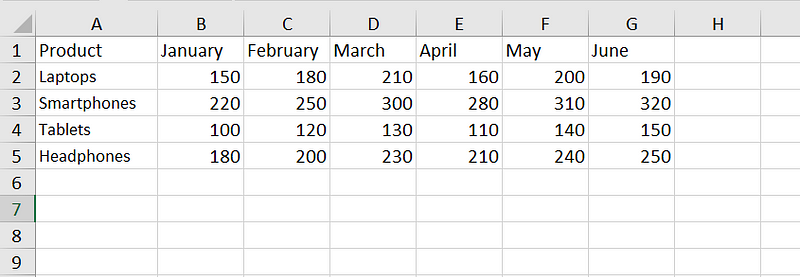
Online retail company sales data. (This and all below images by author)

We’ll see how to use the HLOOKUP function to find the sales figures for “Laptops” in March:

• Step 1: Select a cell where you want to display the result. Here, let’s use cell I2.

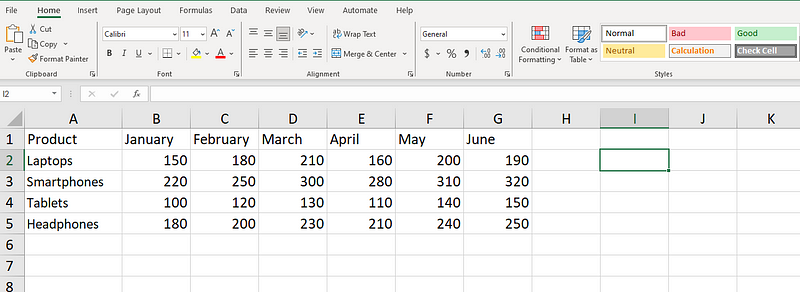
Selecting a cell to perform the HLOOKUP function.

• Step 2: Type the following formula in cell I2:

=HLOOKUP("March", B1:G2, 2, FALSE)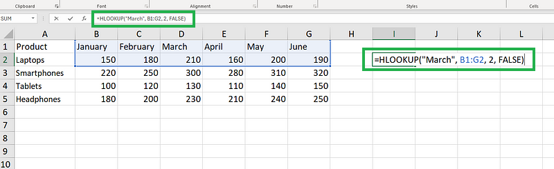

Typing the HLOOKUP formula.

• Step 3: Enter the cell.

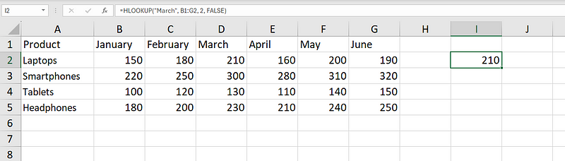
The HLOOKUP function successfully searched for the month “March” in the first row of the specified table_array (B1:G1) and returned the corresponding value from the second row (B2:G2), which is 210.

The parameters we provided were:

• "March" is the lookup_value, the month we want to find the sales figures for.
• B1:G2 is the table_array, the range of cells that contains the data we want to search.
• 2 is the row_index_num, indicating that we want to retrieve the value from the second row of the table_array (where the sales figures for "Laptops" are located).
• FALSE specifies that we want an exact match for the lookup_value

Through this example, we saw how HLOOKUP can be used to efficiently retrieve specific data from a horizontal dataset based on a given criterion.

What if we’re not looking for an exact match in the data?

Using HLOOKUP for an Approximate Match

Consider a scenario where a catering company offers different menu packages for events based on the number of guests.

The pricing for these packages is tiered with specific prices for different guest count brackets. They follow a pricing strategy where the per-person cost decreases with higher guest count brackets, encouraging bookings for more guests.

Their pricing card looks as shown below:

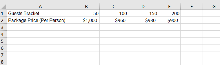
Catering company data.

You have been tasked to find a quick way to determine the total price for any given booking, provided the estimated number of guests, in line with the pricing strategy.

We’ll see how the approximate match parameter of HLOOKUP is handy in such a situation. Let’s follow the earlier steps again:

• Step 1: Select a cell where you want to display the result. Here, we have been given the input (guest count) in call B4, and we would like to display the per-person cost in cell B5. The total cost can be calculated in B6, a simple multiplication of B4 and B5 (Guest Count* Per Person Price).

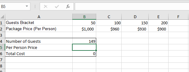
Selecting the cell to perform HLOOKUP.

• Step 2: Type the following formula in cell B4:

=HLOOKUP(B4,B1:E2,2,TRUE)

• Step 3: Enter the cell.

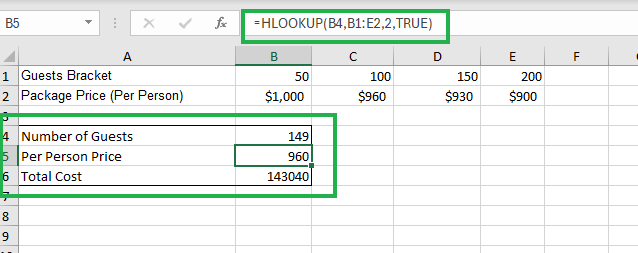
Performing HLOOKUP operation.

After executing the HLOOKUP function in Step 3, cell B5 will display the value of $960. This is the per-person price for the guest count of 149 since it falls in the bracket of above 100 but less than 150.

Here’s the formula we entered:

• B4 has the lookup_value, the guest count for which we want to find the per-person package price.
• B1:E2 is the table_array, the range of cells that contains the data we want to search.
• 2 is the row_index_num, indicating that we want to retrieve the value from the second row of the table_array (where the per-person prices are located).
• TRUE specifies that we want an approximate match since the exact guest count will often vary from our pre-defined brackets.

The HLOOKUP function successfully searched for the nearest guest bracket less than or equal to 149 in the top row of the specified table_array (B1:E1) and returned the corresponding per-person package price from the second row (B2:E2), which is $960.

This example shows us how HLOOKUP with an approximate match is useful in efficiently retrieving data based on a tiered or ranged structure in a horizontal dataset.

Conclusion

This tutorial introduced you to the syntax of HLOOKUP in Microsoft Excel and helped you understand how to use them for your data using multiple examples.

It might seem hard and confusing for the first few times, but once you get used to it, you’ll love the feature and find it convenient to pull data whenever required.

The official Microsoft documentation is always a reliable source of information, in case of any new updates to the tool.

Lastly, for comprehensive learning on leveraging Excel for data analytical skills, check out the Excel Fundamentals track, where you’ll start from being an absolute beginner to building your own customer churn analytics project in Excel.

You can also check out our tutorial on basic Excel formulas and our Excel formulas cheat sheet.