Course
Introduction to Python
4 hr
6.9M

Run and edit the code from this tutorial online
Run codeIf you want to learn more in Python, take DataCamp's free Intro to Python for Data Science course.
You all have seen datasets. Sometimes they are small, but often at times, they are tremendously large in size. It becomes very challenging to process the datasets which are very large, at least significant enough to cause a processing bottleneck.
So, what makes these datasets this large? Well, it's features. The more the number of features the larger the datasets will be. Well, not always. You will find datasets where the number of features is very much, but they do not contain that many instances. But that is not the point of discussion here. So, you might wonder with a commodity computer in hand how to process these type of datasets without beating the bush.
Often, in a high dimensional dataset, there remain some entirely irrelevant, insignificant and unimportant features. It has been seen that the contribution of these types of features is often less towards predictive modeling as compared to the critical features. They may have zero contribution as well. These features cause a number of problems which in turn prevents the process of efficient predictive modeling -
So, what's the solution here? The most economical solution is Feature Selection.
Feature Selection is the process of selecting out the most significant features from a given dataset. In many of the cases, Feature Selection can enhance the performance of a machine learning model as well.
Sounds interesting right?
You got an informal introduction to Feature Selection and its importance in the world of Data Science and Machine Learning. In this post you are going to cover:
Feature selection is also known as Variable selection or Attribute selection.
Essentially, it is the process of selecting the most important/relevant. Features of a dataset.
The importance of feature selection can best be recognized when you are dealing with a dataset that contains a vast number of features. This type of dataset is often referred to as a high dimensional dataset. Now, with this high dimensionality, comes a lot of problems such as - this high dimensionality will significantly increase the training time of your machine learning model, it can make your model very complicated which in turn may lead to Overfitting.
Often in a high dimensional feature set, there remain several features which are redundant meaning these features are nothing but extensions of the other essential features. These redundant features do not effectively contribute to the model training as well. So, clearly, there is a need to extract the most important and the most relevant features for a dataset in order to get the most effective predictive modeling performance.
"The objective of variable selection is three-fold: improving the prediction performance of the predictors, providing faster and more cost-effective predictors, and providing a better understanding of the underlying process that generated the data."
-An Introduction to Variable and Feature Selection
Now let's understand the difference between dimensionality reduction and feature selection.
Sometimes, feature selection is mistaken with dimensionality reduction. But they are different. Feature selection is different from dimensionality reduction. Both methods tend to reduce the number of attributes in the dataset, but a dimensionality reduction method does so by creating new combinations of attributes (sometimes known as feature transformation), whereas feature selection methods include and exclude attributes present in the data without changing them.
Some examples of dimensionality reduction methods are Principal Component Analysis, Singular Value Decomposition, Linear Discriminant Analysis, etc.
Let me summarize the importance of feature selection for you:
In the next section, you will study the different types of general feature selection methods - Filter methods, Wrapper methods, and Embedded methods.
The following image best describes filter-based feature selection methods:

Image Source: Analytics Vidhya
Filter method relies on the general uniqueness of the data to be evaluated and pick feature subset, not including any mining algorithm. Filter method uses the exact assessment criterion which includes distance, information, dependency, and consistency. The filter method uses the principal criteria of ranking technique and uses the rank ordering method for variable selection. The reason for using the ranking method is simplicity, produce excellent and relevant features. The ranking method will filter out irrelevant features before classification process starts.
Filter methods are generally used as a data preprocessing step. The selection of features is independent of any machine learning algorithm. Features give rank on the basis of statistical scores which tend to determine the features' correlation with the outcome variable. Correlation is a heavily contextual term, and it varies from work to work. You can refer to the following table for defining correlation coefficients for different types of data (in this case continuous and categorical).
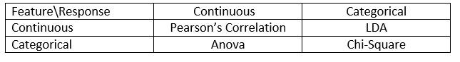
Image Source: Analytics Vidhya
Some examples of some filter methods include the Chi-squared test, information gain, and correlation coefficient scores.
Next, you will see Wrapper methods.
Like filter methods, let me give you a same kind of info-graphic which will help you to understand wrapper methods better:
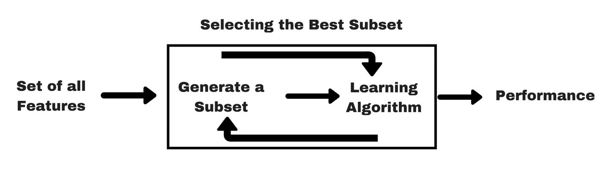
Image Source: Analytics Vidhya
As you can see in the above image, a wrapper method needs one machine learning algorithm and uses its performance as evaluation criteria. This method searches for a feature which is best-suited for the machine learning algorithm and aims to improve the mining performance. To evaluate the features, the predictive accuracy used for classification tasks and goodness of cluster is evaluated using clustering.
Some typical examples of wrapper methods are forward feature selection, backward feature elimination, recursive feature elimination, etc.
Good enough!
Now let's study embedded methods.
Embedded methods are iterative in a sense that takes care of each iteration of the model training process and carefully extract those features which contribute the most to the training for a particular iteration. Regularization methods are the most commonly used embedded methods which penalize a feature given a coefficient threshold.
This is why Regularization methods are also called penalization methods that introduce additional constraints into the optimization of a predictive algorithm (such as a regression algorithm) that bias the model toward lower complexity (fewer coefficients).
Examples of regularization algorithms are the LASSO, Elastic Net, Ridge Regression, etc.
Well, it might get confusing at times to differentiate between filter methods and wrapper methods in terms of their functionalities. Let's take a look at what points they differ from each other.
So far you have studied the importance of feature selection, understood its difference with dimensionality reduction. You also covered various types of feature selection methods. So far, so good!
Now, let's see some traps that you may get into while performing feature selection:
You may have already understood the worth of feature selection in a machine learning pipeline and the kind of services it provides if integrated. But it is very important to understand at exactly where you should integrate feature selection in your machine learning pipeline.
Simply speaking, you should include the feature selection step before feeding the data to the model for training especially when you are using accuracy estimation methods such as cross-validation. This ensures that feature selection is performed on the data fold right before the model is trained. But if you perform feature selection first to prepare your data, then perform model selection and training on the selected features then it would be a blunder.
If you perform feature selection on all of the data and then cross-validate, then the test data in each fold of the cross-validation procedure was also used to choose the features, and this tends to bias the performance of your machine learning model.
Enough of theories! Let's get straight to some coding now.
For this case study, you will use the Pima Indians Diabetes dataset. The description of the dataset can be found here.
The dataset corresponds to classification tasks on which you need to predict if a person has diabetes based on 8 features.
There are a total of 768 observations in the dataset. Your first task is to load the dataset so that you can proceed. But before that let's import the necessary dependencies, you are going to need. You can import the other ones as you go along.
import pandas as pd
import numpy as np
Now that the dependencies are imported let's load the Pima Indians dataset into a Dataframe object with the help of Pandas library.
data = pd.read_csv("diabetes.csv")
The dataset is successfully loaded into the Dataframe object data. Now, let's take a look at the data.
data.head()
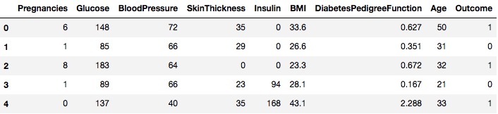
So you can see 8 different features labeled into the outcomes of 1 and 0 where 1 stands for the observation has diabetes, and 0 denotes the observation does not have diabetes. The dataset is known to have missing values. Specifically, there are missing observations for some columns that are marked as a zero value. You can deduce this by the definition of those columns, and it is impractical to have a zero value is invalid for those measures, e.g., zero for body mass index or blood pressure is invalid.
But for this tutorial, you will directly use the preprocessed version of the dataset.
# load data
url = "https://raw.githubusercontent.com/jbrownlee/Datasets/master/pima-indians-diabetes.data.csv"
names = ['preg', 'plas', 'pres', 'skin', 'test', 'mass', 'pedi', 'age', 'class']
dataframe = pd.read_csv(url, names=names)
You loaded the data in a DataFrame object called dataframe now.
Let's convert the DataFrame object to a NumPy array to achieve faster computation. Also, let's segregate the data into separate variables so that the features and the labels are separated.
array = dataframe.values
X = array[:,0:8]
Y = array[:,8]
Wonderful! You have prepared your data.
First, you will implement a Chi-Squared statistical test for non-negative features to select 4 of the best features from the dataset. You have already seen Chi-Squared test belongs the class of filter methods. If anyone's curious about knowing the internals of Chi-Squared, this video does an excellent job.
The scikit-learn library provides the SelectKBest class that can be used with a suite of different statistical tests to select a specific number of features, in this case, it is Chi-Squared.
# Import the necessary libraries first
from sklearn.feature_selection import SelectKBest
from sklearn.feature_selection import chi2
You imported the libraries to run the experiments. Now, let's see it in action.
# Feature extraction
test = SelectKBest(score_func=chi2, k=4)
fit = test.fit(X, Y)

# Summarize scores
np.set_printoptions(precision=3)
print(fit.scores_)

features = fit.transform(X)
# Summarize selected features
print(features[0:5,:])
[ 111.52  1411.887   17.605   53.108 2175.565  127.669    5.393  181.304]
[[148.    0.   33.6  50. ]
 [ 85.    0.   26.6  31. ]
 [183.    0.   23.3  32. ]
 [ 89.   94.   28.1  21. ]
 [137.  168.   43.1  33. ]]
You can see the scores for each attribute and the 4 attributes chosen (those with the highest scores): plas, test, mass, and age. This scores will help you further in determining the best features for training your model.
P.S.: The first row denotes the names of the features. For preprocessing of the dataset, the names have been numerically encoded.
Next, you will implement Recursive Feature Elimination which is a type of wrapper feature selection method.
The Recursive Feature Elimination (or RFE) works by recursively removing attributes and building a model on those attributes that remain.
It uses the model accuracy to identify which attributes (and combination of attributes) contribute the most to predicting the target attribute.
You can learn more about the RFE class in the scikit-learn documentation.
# Import your necessary dependencies
from sklearn.feature_selection import RFE
from sklearn.linear_model import LogisticRegression
You will use RFE with the Logistic Regression classifier to select the top 3 features. The choice of algorithm does not matter too much as long as it is skillful and consistent.
# Feature extraction
model = LogisticRegression()
rfe = RFE(model, 3)
fit = rfe.fit(X, Y)
print("Num Features: %s" % (fit.n_features_))
print("Selected Features: %s" % (fit.support_))
print("Feature Ranking: %s" % (fit.ranking_))
Num Features: 3
Selected Features: [ True False False False False  True  True False]
Feature Ranking: [1 2 3 5 6 1 1 4]
You can see that RFE chose the top 3 features as preg, mass, and pedi.
These are marked True in the support array and marked with a choice “1” in the ranking array. This, in turn, indicates the strength of these features.
Next up you will use Ridge regression which is basically a regularization technique and an embedded feature selection techniques as well.
This article gives you an excellent explanation on Ridge regression. Be sure to check it out.
# First things first
from sklearn.linear_model import Ridge
Next, you will use Ridge regression to determine the coefficient R2.
Also, check scikit-learn's official documentation on Ridge regression.
ridge = Ridge(alpha=1.0)
ridge.fit(X,Y)
Ridge(alpha=1.0, copy_X=True, fit_intercept=True, max_iter=None,
   normalize=False, random_state=None, solver='auto', tol=0.001)
In order to better understand the results of Ridge regression, you will implement a little helper function that will help you to print the results in a better so that you can interpret them easily.
# A helper method for pretty-printing the coefficients
def pretty_print_coefs(coefs, names = None, sort = False):
    if names == None:
        names = ["X%s" % x for x in range(len(coefs))]
    lst = zip(coefs, names)
    if sort:
        lst = sorted(lst,  key = lambda x:-np.abs(x[0]))
    return " + ".join("%s * %s" % (round(coef, 3), name)
                                   for coef, name in lst)
Next, you will pass Ridge model's coefficient terms to this little function and see what happens.
print ("Ridge model:", pretty_print_coefs(ridge.coef_))
Ridge model: 0.021 * X0 + 0.006 * X1 + -0.002 * X2 + 0.0 * X3 + -0.0 * X4 + 0.013 * X5 + 0.145 * X6 + 0.003 * X7
You can spot all the coefficient terms appended with the feature variables. It will again help you to choose the most essential features. Below are some points that you should keep in mind while applying Ridge regression:
Well, that concludes the case study section. The methods that you implemented in the above section will help you to understand the features of a particular dataset in a comprehensive manner. Let me give you some critical points on these techniques:
In this post, you covered one of the most well studied and well researched statistical topics, i.e., feature selection. You also got familiar with its different variants and used them to see which features in a dataset are important.
You can take this tutorial further by merging a correlation measure into the wrapper method and see how it performs. In the course of action, you might end up creating your own feature selection mechanism. That is how you establish the foundation for your little research. Researchers are also using various soft computing principles in order to perform the selection. This is itself a whole field of study and research. Also, you should try out the existing feature selection algorithms on various datasets and draw your own inferences.
Yes, this question is obvious. Because there are neural net architectures (for example CNNs) which are quite capable of extracting the most significant features from data but that too has a limitation. Using a CNN for a regular tabular dataset which does not have specific properties (the properties that a typical image holds like transitional properties, edges, positional properties, contours etc.) is not the wisest decision to make. Moreover, when you have limited data and limited resources, training a CNN on regular tabular datasets might turn into a complete waste. So, in situations like that, the methods that you studied will definitely come handy.
The following are some resources if you would like to dig more on this topic:
Below are the references that were used in order to write this tutorial.
Be sure to post your doubts in the comments section if you have any!
Python Courses
Course
Course
Course
Tutorial
Matthew Przybyla
Tutorial
Kurtis Pykes
Tutorial
Avinash Navlani
Tutorial
Karlijn Willems
Tutorial
Avinash Navlani
Tutorial
DataCamp Team