How to Change Date Format in Excel: What You Need to Know

You download a report from a website, open it in Excel, and every date has turned into a five-digit number. Or worse, you're looking at a mix of U.S. and European date formats in the same column. 

One says 03/07/2025, and you’re wondering: is that March 7th or July 3rd?

If that’s ever made you question your own data, it’s okay because we all have been through this. 

Excel is a helpful software, but its default handling of dates is not always intuitive. In this tutorial, we’ll walk you through how to change date formats in Excel and how to avoid those common and annoying mistakes when importing messy data. 

Understanding Excel's Date Management

At the backend, Excel has its way of storing and interpreting dates. And if you’re not aware of how it works, you may end up making mistakes when sharing files or working across systems. 

So let’s see how it all works.

Serial number architecture

Excel stores dates as serial numbers. For example, January 1, 1900, is stored as the number 1, January 2, 1900, is 2, and so on. This makes it easy for Excel to calculate things like the number of days between dates.

However, there are two date systems:

1. 1900 system: It starts counting from January 1, 1900 (the default on Windows). 
2. 1904 system: It starts from January 1, 1904, and it’s used mostly on Macs.

If you open a file created with one system on a machine using the other, the dates might shift by about four years. 

For example, a date entered as 01/01/2025 on a Mac might display as 01/01/2021 when opened on a Windows PC, because the two systems use different starting points.

This can cause serious confusion. So if you're sharing workbooks across platforms, check which date system the file uses.

Regional settings integration

Excel follows your computer’s regional settings when displaying dates. 

For example, in the U.S., dates are usually written as month/day/year, so 03/07/2025 means March 7, 2025. However, in many other countries, such as the U.K. or Australia, the format is day/month/year. So 03/07/2025 would be read as July 3, 2025.

Suppose you send an Excel file to someone in a different country. Now, if their computer is set to a different regional format, the same date in your file may appear differently on their end, and the formulas can throw errors even if the date hasn’t changed. 

That’s why I‘d recommend double-checking date formats or using clear formats like full month names (e.g., July 3, 2025) when sharing files across regions.

How Excel interprets two-digit years

When we type something like 25 as a year into a date, Excel has to decide whether we mean 1925 or 2025. 

By default, it assumes that:

• If the year is between 00 and 29, it means 2000 to 2029.

• If the year is between 30 and 99, it means 1930 to 1999.

So if we type 4/5/25, Excel will treat it as April 5, 2025, and not 1925. But if we type 4/5/30, Excel will show April 5, 1930.

This rule comes from your Windows settings, not Excel itself. You can change it, but it affects all programs on your computer, not just Excel.

So, I’d recommend using four-digit years instead of changing the setting, as this keeps everything clear and organized. 

Applying Predefined Date Formats

If you don’t like the default date format in Excel, there are tons of date styles you can choose from, depending on how you want the data to look. Let’s see some of these options:

Format cells dialog implementation

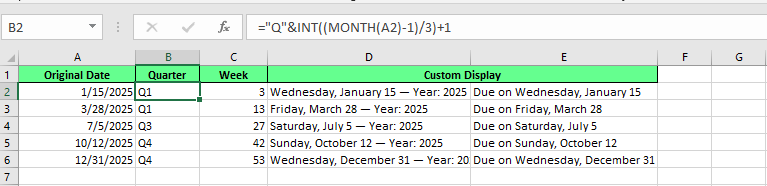
The Format Cells dialog option is easy. Here’s how you can use it: 

1. Right-click on the cell or range of cells with the dates and choose Format Cells. 

2. Press Ctrl+1, an Excel shortcut key. The Format Cells dialog box will appear

3. Under the Number tab, click on Date from the available list.

4. Choose your desired date format from the available options and click OK to apply it.

You'll see a variety of predefined date formats. But before applying a format, take a quick look at the Sample box (as shown in the image below). This shows how your date will look with the selected format. 

Change the date format using the Format Cell dialog box. Image by Author.

Home tab quick formatting

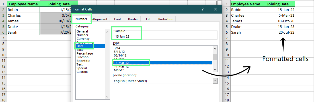
You can also use the Home tab for quick formatting. All you have to do is:

1. Select your cells and go to the Number group. 
2. Click the dropdown. 
3. Now choose Short Date or Long Date (I used a long date in the example below).

This is a faster way to format a date dataset, but it has more limitations. You only have two basic options, and you can’t control details such as how the month or day appears. If you want more options to choose from, it’s better to use the Format Cells dialog.

Change the date format using the Home tab. Image by Author.

Creating Custom Date Formats

If you don't want to use the predefined Excel date formats, you can customize one according to your needs. 

Syntax and code components

Custom date formats use special codes to instruct Excel on how to display each part of the date: 

For example:

And you can combine these in any order to create the exact format you want. You can also use delimiters like dashes, slashes, and commas, however you want. For example: 

To set the syntax of your custom format: 

1. Select the cell or range of cells, and open the Format Cell dialog box with the Ctrl+1 shortcut key. 

2. Under the Number tab, select the Custom option.

3. Now, write the format in the Type field as shown in the image below. 

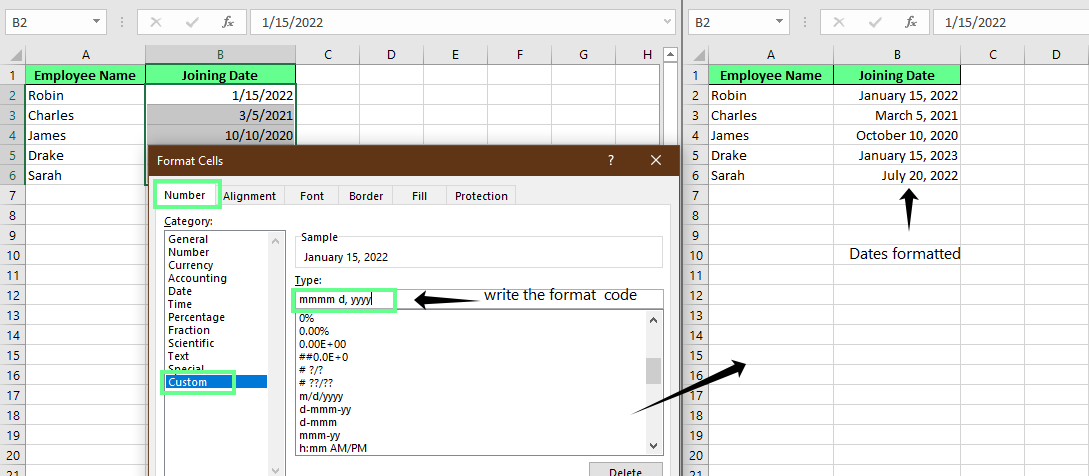
Customize the date format. Image by Author.

That’s it. Your custom date format syntax is set now. 

Custom formats for different locales

You can also create custom formats for different regional conventions.

Even better, you can force Excel to use a specific locale so the format adjusts to a country’s language or date style. 

To do so, add a locale code at the beginning of your format inside brackets, like this:

• [$-409]dddd, mmmm d, yyyy — this uses U.S. English.

• [$-804] for Chinese.

• [$-407] for German, and so on. 

You can check more codes here.

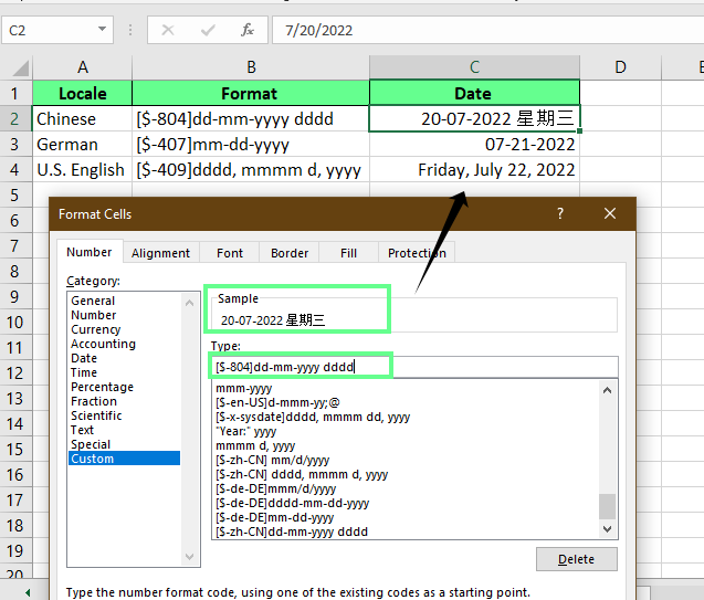
Customize the date format according to different locales. Image by Author.

Advanced customization scenarios

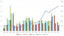
Sometimes you need to go beyond standard dates. For example, you want to display the fiscal quarter, such as Q1 or Q3, based on the date. Or you may need to display the week number of the year.

While Excel doesn’t support these directly through custom date codes, you can combine formulas with custom formats to get the result. 

Here’s how:

• To show the quarter: use a formula like ="Q"&INT((MONTH(A1)-1)/3)+1. This will display the quarter number of the year. If you want to write as Quarter 1, change the formula to ="Quarter "&INT((MONTH(A2)-1)/3)+1

• To show the week number, use =WEEKNUM(A1). This displays the week number of the year. 

In addition, you can add text literals directly into your format using double quotes. For example:

=TEXT(A2, "dddd, mmmm d") & " — Year: " & TEXT(A2,"yyyy")

This will show the date in a readable sentence, like: Saturday, July 5 — Year: 2025

Or, you can even add text like “Due on:”

=TEXT(A2, """Due on"" dddd, mmmm d")

By doing so, Excel treats the words “Due on” as plain text, then follows it with the full day and date in cell A2.

Display Quarters instead of standard dates. Image by Author 

Note: Be careful with formatting codes. m can mean month or minute, depending on where you use it. 

• If it comes after an hour, code like h (h: mm) will be treated as minutes in Excel. 

• If it comes after a day or (mm/dd/yyy), it means a month.

Managing and Converting Non-Date Entries

Not everything that appears to be a date in Excel is, in fact, a date. Sometimes, dates are entered as plain text, which can cause problems when you attempt to format or calculate with them.

Converting text to dates

When you copy data from other systems, such as CSV files or databases, the cell with dates may appear to be a date, but Excel treats it as plain text, not an actual date.

To fix this, you can use two methods:

1) DATEVALUE function

This function takes a date stored as text and converts it to a real Excel date.

For example, in cell A1, the date 07/05/2025 is written as text. To solve this, we use:

=DATEVALUE(A2)

This returns the serial number for that date. Then I formatted it back to date using the options discussed above.

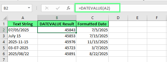
Convert text to a date using DATEVALUE(). Image by Author.

2) Text-to-Columns tool

You can also use the text-to-columns feature to convert text to dates. Here’s how:

• Select the column with text dates. 
• Go to the Data tab, then click Text to Columns.
• Select the Delimited option, then click Next.
• Select the Delimiter, then click Next.
• Select Date, and pick the format (like MDY). 
• Select the Destination where you want to display the result and click Finish.

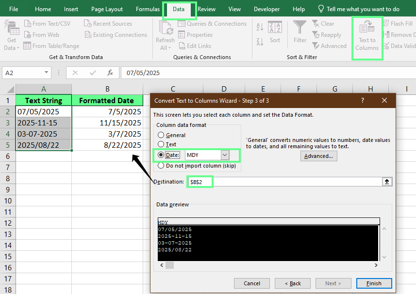
Convert text to date using the Text to Column wizard. Image by Author.

That’s it. You can see that Excel instantly converted all the text entries to real dates.

Persistent formatting challenges

Sometimes, even after trying these methods, Excel still refuses to treat the data like a proper date. These are what we call stubborn text dates.

This often happens because:

• The delimiter is wrong (using dashes when Excel expects slashes).
• The regional settings on your system don’t match the format of the incoming data.
• Or extra spaces or invisible characters are stuck in the cells.

To fix this:

Use the TRIM() function to remove hidden spaces:

=TRIM(A1)

Or use SUBSTITUTE() to replace dashes with slashes if needed:

=DATEVALUE(SUBSTITUTE(A1,"-","/"))

Let’s say Excel doesn’t recognize 5th July 2025 as a date. So you can remove the th from it like this: 

=SUBSTITUTE(A1,"5th","5")

Converting dates to numbers

Behind every Excel date is a serial number. Excel uses this to perform date math, such as calculating the number of days between two dates.

To see this number: 

• Click the date cell.
• Go to the Number group in the Home tab.
• Select General or Number. 

The date July 5, 2025 will show as 45843.

You can also use formulas instead of finding it manually:

• =DATEVALUE("7/5/2025") display 45843.

• =TIMEVALUE("10:30 AM") returns a decimal value, such as 0.4375, because time is part of a full day.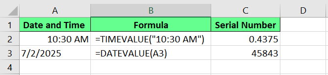

Convert dates to numbers. Image by Author.

Useful Excel Date Formulas for Managing Dates

Excel has built-in date formulas that can save you time and make your spreadsheets more dynamic. If you want to track deadlines or prepare reports, these formulas can help automate your workflow.

Common date-related formulas

Here are some of the most commonly used date functions:

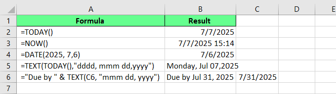
Date-related built-in formulas. Image by Author.

Data preparation and display tips

In Excel, clarity and consistency are everything, especially if your file is going to be shared or used in reporting. A few simple habits can go a long way in preventing confusion and formula errors. 

Here are some quick tips to keep your dates clean, readable, and reliable:

• Always use full four-digit years (e.g., 2025 instead of 25) to avoid confusion or misinterpretation.

• Always use a consistent date format throughout the sheet, such as mm/dd/yyyy or dd-mmm-yyyy. 

• Use TEXT() to create friendly labels in dashboards and charts. 

• If you import messy data, use one column for the raw value and another with a formula to convert or format it.

Configuring System-Level Date Settings

Excel uses your computer’s system date settings to decide how dates are displayed. By adjusting these settings, you can control how Excel shows dates by default, whether for personal use or across an entire organization.

Regional default overrides

Excel uses the regional settings from Windows to format dates. If you want Excel to display dates in a specific format by default, you can adjust your system settings. 

Here’s how:

1. Open the Control Panel from the Start menu. 
2. Go to Clock and Region (may differ in some systems) and then select Region. 
3. Select the region and choose the date format from the drop-down lists. 
4. Once done, click Apply.

However, if you prefer not to use the predefined format and would like to customize it yourself, use the Additional Settings option.

1. Under the Date tab, set your preferred Short and Long date formats. 
2. Hit Apply.

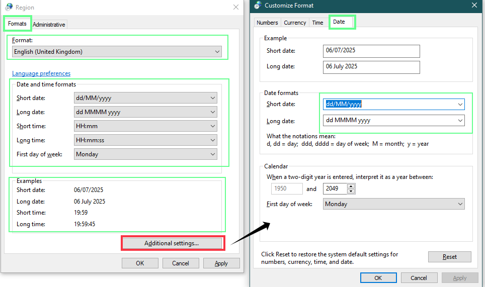
Change the regional setting in Windows. Image by Author

Asterisk vs. non-asterisk formats

When you choose a date format in Excel (through Format Cells), you’ll notice some have an asterisk ( * ) in front of them, like this:

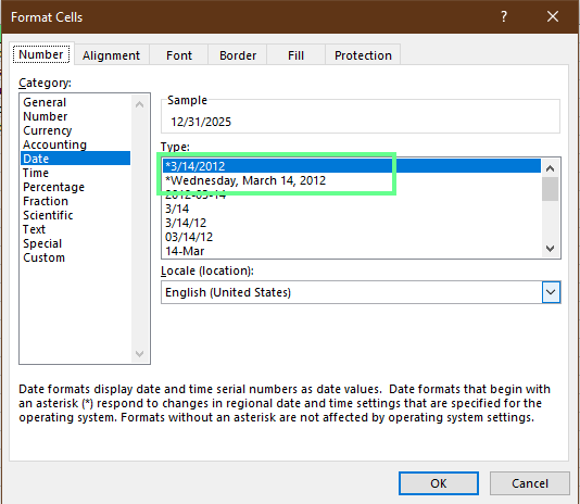
Default date format. Image by Author.

These asterisk formats are linked to your Windows regional settings, and they’ll automatically update if you change your system format.

But formats without an asterisk are fixed—they won’t change, no matter what your system settings are.

Note: Use asterisk formats if you want your file to adjust to the user’s system settings. But use non-asterisk formats if you want the date's appearance to remain consistent, regardless of where it's displayed.

Enterprise deployment strategies

In organizations, consistency is important, primarily when teams work across different locations or systems. You don’t want one team using MM/DD/YYYY and another using DD/MM/YYYY in the same report.

Here are a few ways IT teams or Excel power users can manage this:

1. Use Group Policy to control system date settings.

Group Policy is a Windows feature that allows administrators to control settings across all computers in a company or network. Instead of asking each user to change their settings manually, admins can apply rules that update or lock settings for everyone automatically.

Let’s say your company is based in the UK. You want all Excel users to see and enter dates in the format DD/MM/YYYY.

With Group Policy, an admin can:

• Set the system date format on all employee computers.
• Lock that setting so users don’t accidentally change it.
• Ensure that Excel uses this format by default (via the asterisk-linked formats).

2. Provide standardized Excel templates.

You can also create and share Excel templates with:

• Pre-set date formats
• Sample date formatting instructions
• Protected cell formatting to prevent accidental changes

This is a simple yet effective way to ensure every team member starts with the same structure and formatting rules.

Troubleshooting Common Date Formatting Issues

Here are some of the most common date-related issues and how to fix them.

Display and fit errors

If you write the date in a cell, it shows #####. This means that the cell is too narrow to show the full date value. So you need to expand your cell. 

To do so, double-click the right edge of the column header or drag it manually.

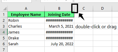
Expand the column. Image by Author.

Another issue is when negative numbers accidentally turn into strange-looking dates. This happens when the cells were previously formatted as a date, and a negative number goes in (like -1), so it turns into a date 

To fix this, change the cell format back to General or Number using the Home tab > Number Format dropdown.

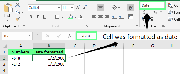
Fix negative numbers that display as dates. Image by Author.

Import and copy-paste discrepancies

Excel may treat your dates as plain text instead of real date values, as we discussed above.

To fix this, you can:

• Use the Text-to-Columns feature (under the Data tab) to convert text into actual dates.

• Use =DATEVALUE() if the format is readable (e.g., 07/05/2025).

Another issue occurs when we copy and paste between different Excel files (especially between Windows and Mac). You may notice that the date shifts forward or backward by 4 years. This happens because one file uses the 1900 date system, and the other uses the 1904 system.

To fix this: Go to File > Options > Advanced > When calculating this workbook. Then, check or uncheck Use  1904 date system, depending on your source.

Locale and system mismatch errors

When we work with people in different countries, formats can be confusing, such as when one person’s system uses MM/DD/YYYY and another uses DD/MM/YYYY. 

If someone enters 04/05/2025, Excel may read it as April 5 on a U.S. system but May 4 on a U.K. system.

To fix this:

• Use clear, full formats with month names, like 5 July 2025, to avoid confusion.

• Or use TEXT() functions to create a clear, fixed display like this:

=TEXT(A1, "dd-mmm-yyyy")

This displays the dates as 05-Jul-2025, which is compatible across systems.

Conclusion and Best Practices

Excel’s date formatting quirks can quietly derail collaboration and reporting. Especially when you're working across systems (Windows vs. Mac), languages, or time zones.

To avoid surprises, build with global workflows in mind. Use clear, locale-neutral formats (like ISO: yyyy-mm-dd) and document formatting choices directly in your workbook. It’s a small step that pays off.

In short, treat date formatting as a design decision rather than a setting, as a bit of intentionality here keeps your spreadsheets clean and collaborative.