
Course
Introduction to Excel
4 hr
237.2K
There are a couple of different methods to find the days between dates in Excel. They are functionally mostly the same. I'll show each method and you can find the one you like the best.
Simple subtraction is one of the easiest and quickest ways to find the days between the dates. It subtracts one date from another date. Its syntax is:
New date - Old dateHere, I have a dataset with dates in cells A2 and B2, and in cell C2, I enter the following formula:
=B2-A2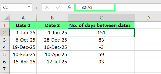
Find days between dates using the subtraction method. Image by Author.
Another way I’ve done it is with the DAYS() function, specifically designed for this. Its syntax is:
=DAYS(end_date, start_date)In the cell C2, I enter the following formula:
=DAYS(B2,A2)Like subtraction, if the end date is after the start date, the result is positive. If it’s before, it’s negative.
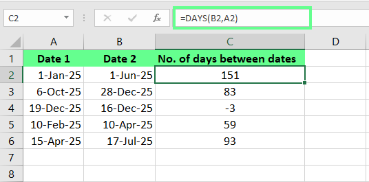
Find days between dates using the DAYS() function. Image by Author.
Like the DAYS() function, DATEDIF() subtracts dates, but the order of the arguments is reversed. Its syntax is:
=DATEDIF(start_date, end_date, "d"))The third argument specifies the unit of time. For example, d is for days, y for years, and m for months.
In cell C2, I entered the following formula:
=DATEDIF(A2, B2, "d")However, when I pressed Enter, I got a #NUM! error in the third row. That’s because the formula tries to subtract a newer date (end_date) from an older date (start_date) and the DATEDIF() function doesn’t allow this. So while DATEDIF() is more flexible it allows for different units of time, it's also less flexible because it doesn't return negative results.
Note also that DATEDIF() is a hidden function, so Excel doesn’t suggest it as I type. This means you’d have to type everything manually if you’re using this function.
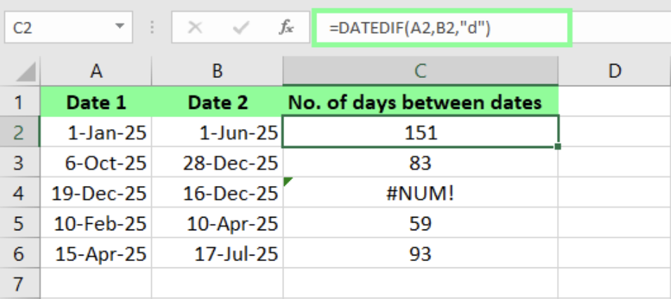
Find the days between the dates using the DATEDIF() function. Image by Author.
NETWORKDAYS() and NETWORKDAYS.INTL() functions only find working days and exclude weekends and holidays. Let's say you want to know the number of working days between two dates and exclude weekends. In this case, you can use the NETWORKDAYS() function to skip Saturdays and Sundays automatically. Its syntax is:
NETWORKDAYS(start_date, end_date, [holidays])For example, if I don’t specify any holidays, it only excludes weekends. In cell C2, I enter the following formula:
=NETWORKDAYS(A2,B2)This gives me the number of working days between the dates in A2 and B2, excluding weekends.
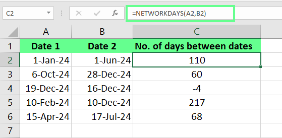 Find the days between the dates using NETWORKDAYS() function. Image by Author.
If I also want to exclude holidays, I list those dates in a separate column like E2 to E5. Then, I reference that range in the third argument like this:
=NETWORKDAYS(A2,B2,$E$3:$E$4)Now, it calculates the working days, excluding both weekends and the holidays I’ve listed. This makes it super easy to get an accurate count of workdays.
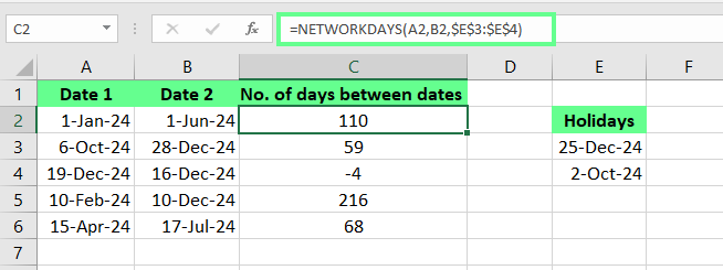
Using NETWORKDAYS() function. Image by Author.
Sometimes, my weekends aren’t the default Saturday and Sunday. In that case, I use the NETWORKDAYS.INTL() function. This lets me define custom weekends. Its syntax is:
NETWORKDAYS.INTL(start_date, end_date, [weekend], [holidays])For the weekend argument, I can either use a number to pick a preset weekend (like 1 for Saturday-Sunday or 7 for Friday-Saturday) or even use a custom text string like 0000011, where each digit represents a day of the week (starting with Monday). 1 marks it as a weekend, and 0 as a working day.
Suppose my weekends are Friday and Saturday. For that, I will use this formula:
=NETWORKDAYS.INTL(A2, B2, 7, $E$2:$E$3)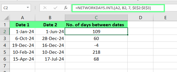 Find the days between the dates using NETWORKDAYS.INTL(). Image by Author.
If I want to calculate how many days have passed since a specific date or how many days are left until a future date, I always use the TODAY() function. This function returns the current date, so I don’t have to update it daily. Its syntax is:
=TODAY() - past_dateLet’s say the past date is in cell A3. So, I enter this formula in cell B3:
=TODAY()-A3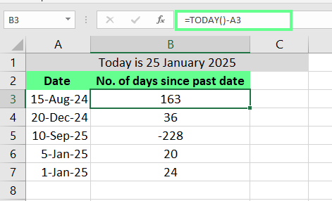
Find the days left since the date with the TODAY() function. Image by Author.
If I need to know how many days are left until a future date, I just flip the formula:
=Future_date - TODAY()So it’d become:
=A3 - TODAY()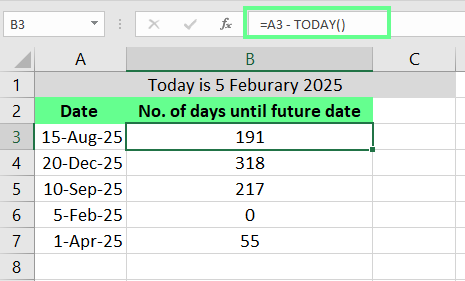
Find the days left until the date with the TODAY() function. Image by Author.
| Method | What I like | What I don’t like |
|---|---|---|
| Simple subtraction | Quick and easy | It doesn’t account for weekends or holidays |
| DAYS() | Clear and structured syntax | It only works for days |
| DATEDIF() | Flexible for days, months, or years | Throws an error when the value is negative |
|
NETWORKDAYS() NETWORKDAYS.INTL() |
Excludes weekends and holidays | Requires extra setup for holidays |
| TODAY() | Updates automatically every day | It only works for calculations involving the current day |
Apart from basics, if you handle complex scenarios, here are some advanced techniques:
When the order of dates is reversed, we get a negative value. To fix it, I wrap the DAYS() function inside the ABS() function like this:
=ABS(DAYS(B2,A2))And you can see the results in the image below:
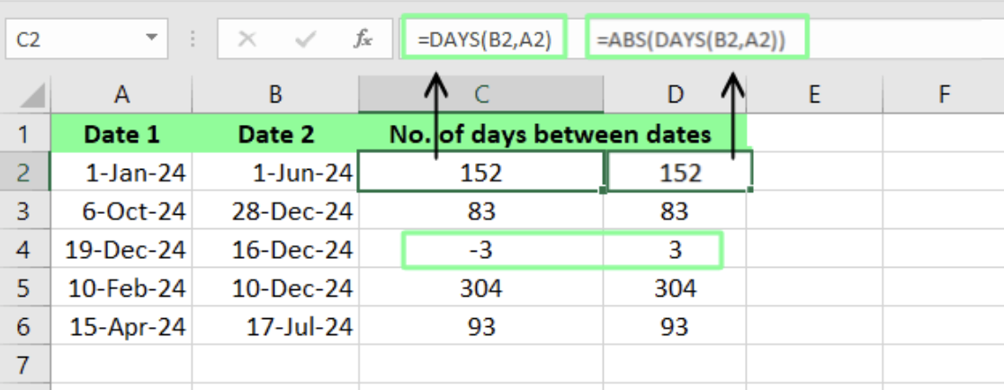
Use the ABS() function to handle negative values. Image by Author.
Here are common Excel date errors I’ve faced and how I fixed them.
#VALUE! error: This happened when my system was set to mm/dd/yyyy for dates, but my formula was using dd/mm/yyyy. I fixed it by updating the dates in the formula to match the format of my system.
#NUM! error: I got this error while using the DAYS() function, and it was because one of the dates had a numeric value outside the valid range for dates. To avoid this, make sure the value is in the valid range.
#NAME? error: This is usually a typo issue (DATEIF() instead of DATEDIF()). To avoid such issues, double-check your spelling.
Sometimes, a single date function isn’t enough for complex tasks, so I combine multiple functions to create a dynamic formula that handles different scenarios.
Suppose I want to figure out how many school days are left until exams. For this, I use NETWORKDAYS() to count working days and add IFERROR() to handle invalid dates. In this case, the formula would look like this:
=IFERROR(NETWORKDAYS(TODAY(), A2, $B$3:$B$4), "Check Dates")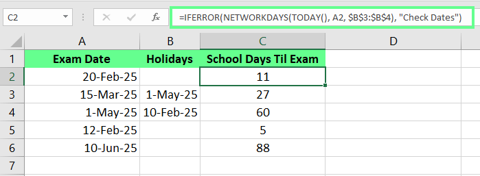
Combine IFERROR() with NETWORKDAYS. Image by Author.
Let me share a few real-life examples of how I recently used these functions in my projects.
I was given a list of dates to calculate the age of individuals based on their dates of birth. To do so, I used the DATEDIF() function. You can see the sample dataset below. In cell B2, I enter
=DATEDIF(A2,TODAY(),"Y")This formula then calculates the number of full years between the date in A2 (date of birth) and today’s date.
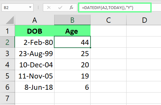
Find the age using the DATEDIF() function. Image by Author.
If I need more specific details, like the total months or days, I can adjust the formula like this:
m to find the number of months since birth.
d to find the number of days.
I also tracked the working days left for a project with the NETWORKDAYS() function. To do so, I entered the start and end dates in cells A2 and B2 and listed the holidays in cells C2:C5. Then, to calculate the working days for the project, I entered the formula in cell D2:
=NETWORKDAYS(A2,B2,$C$3:$C$5)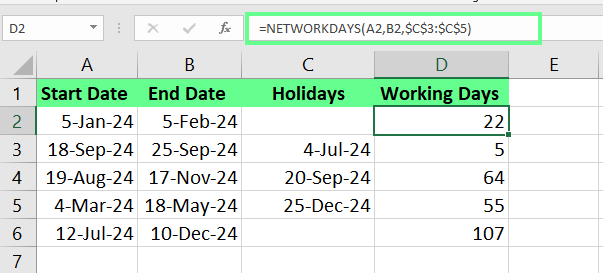
Find the days left for the project using NETWORKDAYS() functions. Image by Author.
Whenever the project timeline changed, I just update the dates, and the formula would adjust automatically. This way, I can easily keep track of the deadlines.
Once, I had to track multiple contract deadlines. So, I set up a simple system in Excel to make it easier to identify an expired or active deadline.
I simply entered this formula in cell C2:
=IF(B2 < TODAY(), "Expired", "Active")This labeled each contract automatically based on whether its expiration date had passed.
I even use conditional formatting to color-code the cells based on their status for clarity. Active contracts are highlighted in green, while Expired contracts are marked in red.
To do so, I selected New Rule under the Conditional Formatting, and chose Use a formula to determine which cells to format. Then, I entered the formulas =B2="Expired" and =B2="Active" separately. This way, I was able to identify which contracts need attention.
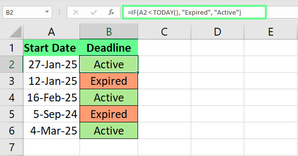
Track the contract deadline. Image by Author.
Now, everything updates on its own. The formulas adjust instantly whenever I add new contracts or update expiration dates.
One could also calculate the gap between prescription refills in Excel. Let’s say your parents picked up a 30-day supply of medication on January 1, 2025, but today is February 5, 2025, and you are trying to figure out how long they went without medication.
In the dataset below, cell A2 shows when the medication was last picked up. We simply subtract today from that date and add 30. (This is just an example for the purpose of practicing Excel functions, and for medical situations, consult your doctor.)
=TODAY()-(A3+30)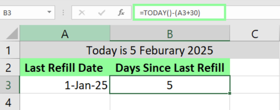
Find the last medication refill. Image by Author
This way, I easily tracked the number of days since each refill and planned the next one without any guesswork.
Now, here are a few tips and best practices to help you along the way:
I always ensure the date cells are formatted correctly. If they’re not, Excel may not recognize them as dates, which can mess up the calculations. So, I always double-check that the cells are set to the Date from the Home tab under the Name group format.
I keep my formulas simple and clear. Instead of hardcoding dates like =DAYS("1/10/2025", "1/1/2025"), I always use cell references like A2 and B2. This way, if I ever need to update the dates, I just change the cell values without touching the formula.
When using the TODAY() function, I always make sure the cell is formatted to Number format — otherwise, it will show a #### error or incorrect date.
I’ve shared some of the best ways to work with dates in Excel, from simple subtraction to more advanced functions like DAYS(), DATEDIF(), NETWORKDAYS(), and TODAY(). These functions are great for tracking timelines and managing holidays.
The best way to get comfortable with these is by practicing. Try them out in your own spreadsheets and see how they can simplify your work.
If you’re ready to take your skills even further, I recommend taking the Data Analysis in Excel course, Data Preparation in Excel course, and Data Visualization in Excel course. These courses cover advanced features and strategies that can make your work even more efficient.
Gain the skills to maximize Excel—no experience required.
Learn Excel with DataCamp
Course
Course
Course
Tutorial
Allan Ouko
Tutorial
Vinod Chugani
Tutorial
Laiba Siddiqui
Tutorial
Travis Tang
Tutorial
Laiba Siddiqui
Tutorial
Samuel Shaibu