How to Combine VLOOKUP() with IF() in Excel

If you manage large datasets in Excel, you know how challenging it is to organize and analyze them efficiently. But I’ve got a solution for you: You can nest the VLOOKUP() function inside an IF() statement to create dynamic lookups based on specific conditions. Using this approach, you can look up different tables based on a condition and you can also handle errors more gracefully.

To be specific, VLOOKUP() finds specific data points within a table, and IF() statements allow you to make conditional decisions based on that data. Both functions are, as we know, extremely important. In this article, we will add another tool to the toolbox: You will learn how you can leverage the power of both of these functions together to perform conditional lookups, and we will illustrate with practical examples.

The Quick Answer: How to Combine VLOOKUP() and IF()

To create a conditional lookup, start with an IF() statement and use VLOOKUP() inside it to return different results based on a condition. We can use the following code to check if a product is in stock based on its quantity. Just follow these steps:

• Start with the IF() function: =IF()

• Inside the IF() function, use VLOOKUP().

=IF(VLOOKUP(C2, $A$2:$B$6, 2, FALSE) > 0, "In Stock", "Out of Stock")

Understanding VLOOKUP() and IF() Statements in Excel

VLOOKUP() helps you find data in a table, while IF() statements let you decide based on that data. Together, they help analyze information in spreadsheets. Let’s look at each function separately and then bring them together. 

What is VLOOKUP() in Excel?

VLOOKUP() searches for a specific value in the first column of a range and returns a value from another column in the same row. Here’s the syntax so you can use the VLOOKUP() formula for your large datasets.

=VLOOKUP(search_key, range, index, is_sorted)

Let’s break down this syntax and understand it:

• Search_key is the value you want to search for. This can be a number, text, or a reference to a cell containing the search value.

• Range defines the range of cells that contains the data. The first column in this range should contain the search_key. 

• Index is the column number in the range from which you want to retrieve the value. The first column is 1, the second is 2, and so on.

• Is_sorted is a logical value (TRUE or FALSE). You can use TRUE (or 1) for numbers and FALSE (or 0) for text. If TRUE, VLOOKUP() assumes that the first column of the range is sorted in ascending order and returns the closest match. If FALSE, VLOOKUP() searches for an exact match. If the argument is not specified, TRUE is the default. 

Let’s understand with an example. Here I have a list of products with their IDs and prices. I want to find the prices for specific products based on their name.

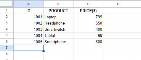
List of products with their ID and prices. Source: Image by Author.

To start, I’m looking to find the price of a tablet specifically. To do this, I enter a search_key value (in my case, Tablet) to find the price in any cell. 

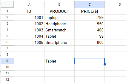
Enter the value to find the price of it. Source: Image by Author.

Then, I select a cell and type =VLOOKUP().

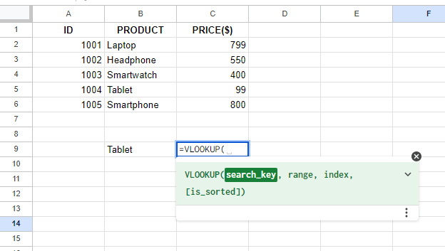
Typing the VLOOKUP() formula. Source: Image by Author.

Next, I select the cell where search_key was entered.

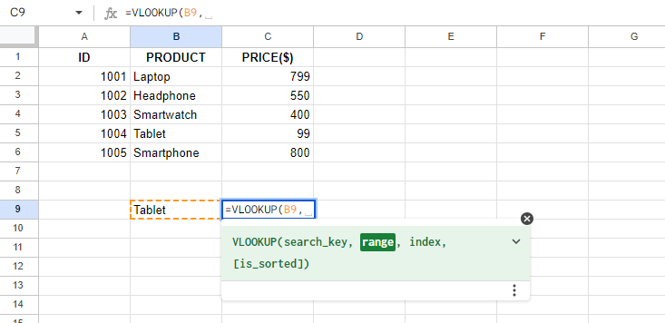
Selecting the column where the product is located. Source: Image by Author.

Then, I select the range of the table. 

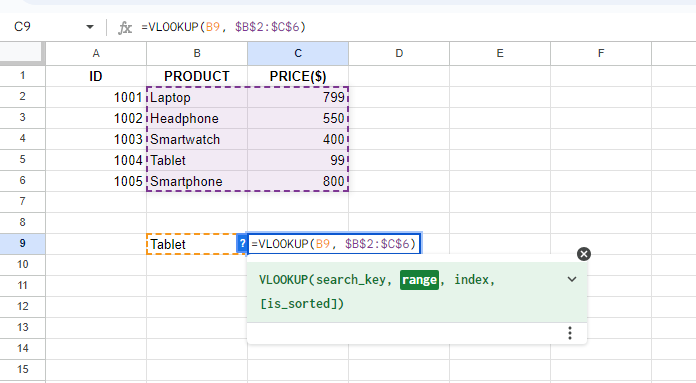
Selecting the range of the table. Source: Image by Author.

Counting from the left, I enter the number of a column from where I wanted to retrieve the data. Here, I want to know the price, so I enter 2.

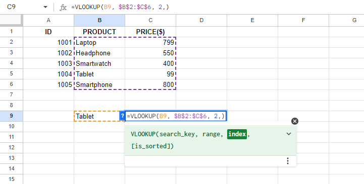
Selecting the index of the columns. Source: Image by Author.

Then, I type FALSE to get the exact match.

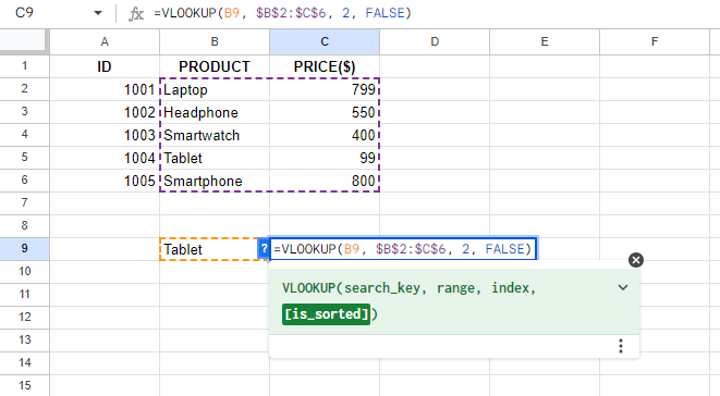
Typing FALSE for the exact match. Source: Image by Author.

After filling all the values, I hit Enter:

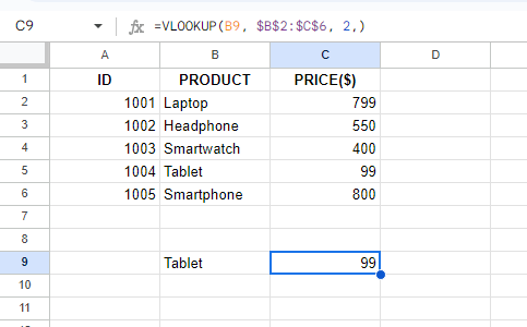
Using VLOOKUP(), the price of the product is achieved. Source: Image by Author.

As you can see in the image, VLOOKUP() successfully retrieves the price.

What is IF() in Excel?

IF() statements compare the values and check them against the specified condition. Here is the syntax:

=IF(logical_test, [value_if_true], [value_if_false])

Let’s look at the key parts to understand it: 

• Logical_test is the value or expression you want to evaluate as TRUE or FALSE. This is the condition you want to check.

• Value_if_true returns the value if logical_test is TRUE.

• Value_if_false returns the value if logical_test is FALSE.

Let’s take an example. Here I want to give remarks to the students based on their grades. So, I prepare the sheet with two columns: STUDENTS and GRADES. 

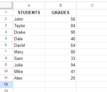
A sheet containing the list of students with their grades. Source: Image by Author.

I select a cell and type =IF(). My goal is to check if the total numbers are greater than 50 and then print Excellent, or, if the grade is less than 50, I print Bad. After specifying the conditions, I hit Enter to get the results.

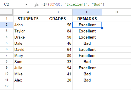
Assigning remarks to all the students using the IF statement. Source: Image by Author.

Then, I copy the formula to the last filled cell by dragging it. You can see the results. I’ve assigned remarks to all the students with just a single formula. 

Ways to Combine VLOOKUP() with IF() in Excel

Let's look into practical examples to understand how VLOOKUP() works with IF().

Conditional lookups

To create a conditional lookup, as we said, start with an IF() statement and use VLOOKUP() inside it to return different results based on a condition.

1. Start with the IF() function: =IF().

2. Inside the IF() function, use VLOOKUP().

Let's try a new example: Here I have a list of product orders with their corresponding order times. I want to see if a specific product has been ordered before 12:00 PM.

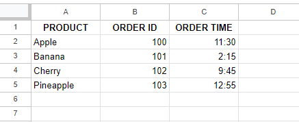
A table containing product list along with order ID and time. Source: Image by Author.

First, I select a column and enter the following formula: 

=IF(VLOOKUP(A3, A2:C5,3, FALSE) < TIME(12, 0, 0), "Ordered Before Noon", "Ordered After Noon")

Here, the VLOOKUP() function looks for Banana in column A and returns the corresponding order time from column B.

The IF() statement checks if the order time is less than 12. If so, it returns Ordered Before Noon. Otherwise, it returns Ordered After Noon.

Calculating the delivery time by combining the IF() and VLOOKUP() formula. Source: Image by Author.

You can see how I easily track my desired product deliveries using conditional lookups.

Error handling

To handle errors, start with an IF() statement and use ISNA() with VLOOKUP() inside it to check for errors. For example, to display a custom message if a product is not found:

1. Start with the IF() function: =IF().

2. Inside the IF() function, use ISNA() with VLOOKUP() to check for errors.

Let’s make this clear with an example. Say I have a table with product prices and I want to display a custom message whenever a product is not found. 

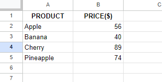
A table containing a list of products and their prices. Source: Image by author.

To do so, I select a cell and enter the following formula to find the price:

=(VLOOKUP(B7, $A$2:$B$5, 2, FALSE)

Then, I combine it with ISNA() and IF() to handle any errors.

=IF(ISNA(VLOOKUP(B7, $A$2:$B$5, 2, FALSE)), "Product Not Found", (VLOOKUP(B7, $A$2:$B$5, 2, FALSE)))

Handling errors by combining IF() and ISNA() formulas. Source: Image by author.

Here, ISNA() checks if the VLOOKUP() function returns an #N/A error, which would happen if is not available. In other words, if ISNA() evaluates to TRUE, the IF() statement returns Product Not Found; otherwise, it returns the price from the VLOOKUP().

Dynamic column indexing

To dynamically choose the column index for VLOOKUP(), start with an IF() statement and use VLOOKUP() inside it to select different columns based on a condition. For example, to look up different columns based on a threshold value:

1. Start with the IF() function: =IF().

2. Inside the IF() function, use VLOOKUP() to check the threshold and select the column.

Here, I have a product table with column A containing the product names, column B containing the product prices, and column C containing the stock quantity. I want to look up the product price or the stock quantity based on whether the price is above or below a certain threshold, like 50.

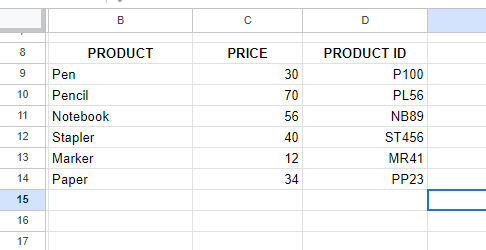
A table containing a list of products, their IDs, and prices. Source: Image by Author.

I select a cell and enter the following formula:

=IF(VLOOKUP(B9, $B$9:$D$14, 2, FALSE) > 50, VLOOKUP(B9,$B$9:$D$14, 3, FALSE), VLOOKUP(B9,$B$9:$D$14, 2, FALSE))

Applying IF with nested VLOOKUP(). Source: Image by Author.

Here’s how the formula works: 

• (VLOOKUP(B9, $B$9:$D$14, 2, FALSE) looks up the product in B9 from column A and returns the price from column C.

• The IF() statement checked if the price is greater than $50.

• If true, our code returns the stock quantity: VLOOKUP(B9,$B$9:$D$14, 3, FALSE).

• If false, our code returns the product ID: VLOOKUP(B9,$B$9:$D$14, 2, FALSE)).

If you’re working with a very large dataset, you can copy the formula by dragging it to the last filled cell.

Showing results. Source: Image by Author.

And that’s it. As you can see, we can retrieve desired information based on specific conditions using a combined formula.

Advanced Techniques Using VLOOKUP() and IF()

Now that you have a basic understanding of combining IF() statements with VLOOKUP(), let’s learn some advanced techniques from examples I tried on my own.

Combining multiple criteria

If you’re looking up data based on multiple criteria, you can combine multiple VLOOKUP() functions within an IF() statement to check if all conditions are met. 

Here I have a table with customer purchase data and membership status. And I want to check if a customer was eligible for a loyalty program, which requires at least 500 in TOTAL PURCHASE ($) and Gold as MEMBERSHIP STATUS.

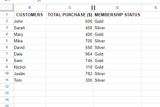
A table containing customers’ details. Source: Image by Author.

I create another column named Eligibility, showing the eligibility criteria. Then, I type the following formula and hit Enter: 

=IF(AND(VLOOKUP(B2, $B$2:$D$11, 2, FALSE) >= 500, VLOOKUP(B2, $B$2:$D$11, 3, FALSE) = "Gold"), "Eligible", "Not Eligible")

Check the eligibility criteria of customers by combining multiple criteria. Source: Image by Author.

Here’s how this formula works: 

• VLOOKUP(B2, $B$2:$D$11, 2, FALSE) >= 500 checks if the customer's total purchases are at least $500.

• VLOOKUP(B2, $B$2:$D$11, 3, FALSE) = "Gold") checks if John's membership status was Gold.

• AND combined the conditions to ensure both are true.

• IF() returned Eligible when both conditions were true. Otherwise, it returned Not Eligible.

Using VLOOKUP() with IF() for calculations

You can use VLOOKUP() to find a value and then apply an IF() statement to perform calculations based on that value. 

Here I prepare a sheet with products and their prices. Then, I want to apply a 10% discount to products above $100.

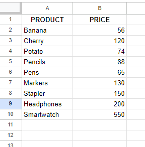
A table containing a list of products with their prices. Source: Image by Author.

So, I create another column named DISCOUNT and I write the following formula in that column to display the discount.

=IF(VLOOKUP(A2, $A$2:$B$10, 2, FALSE) > 100, VLOOKUP(A2, $A$2:$B$10, 2, FALSE) * 0.9, VLOOKUP(A2, $A$2:$B$10, 2, FALSE))

Now, here’s how this formula works:

• VLOOKUP(A2, $A$2:$B$10, 2, FALSE) retrieved the price of the product which is  56.

• =IF(VLOOKUP(A2, $A$2:$B$10, 2, FALSE) > 100, ..., ...) checked if the price of the product was greater than 100. 

• Since the condition is true, VLOOKUP(A2, $A$2:$B$10, 2, FALSE) * 0.9 applied a 10% discount. 

• (VLOOKUP(A2, $A$2:$B$10, 2, FALSE)) printed the actual prices of the product where the discount condition wasn’t true.

That’s how I got the final result of the formula for the product, which was 135. To get the desired results for all products, you can drag down the formula and copy it to the last filled cell.

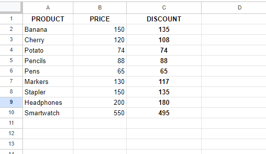
Using VLOOKUP() with IF to calculate the discounts on products whose prices are greater than 100. Source: Image by Author.

Handling large data sets

You can also combine VLOOKUP() with the IF() function to streamline data retrieval and error handling when working with huge datasets.

Here's our final example: I have a sheet with employee information, and I want to retrieve an employee's department and handle cases where the employee ID does not exist.

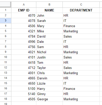
A table containing a list of employees with their IDs and Departments. Source: Image by Author.

So, I select a cell and typed the following formula: 

=IFERROR(VLOOKUP(E3, $A$2:$C$18, 3, FALSE), "Not Found")

After hitting Enter, I drag the formula to copy it to other cells, too.

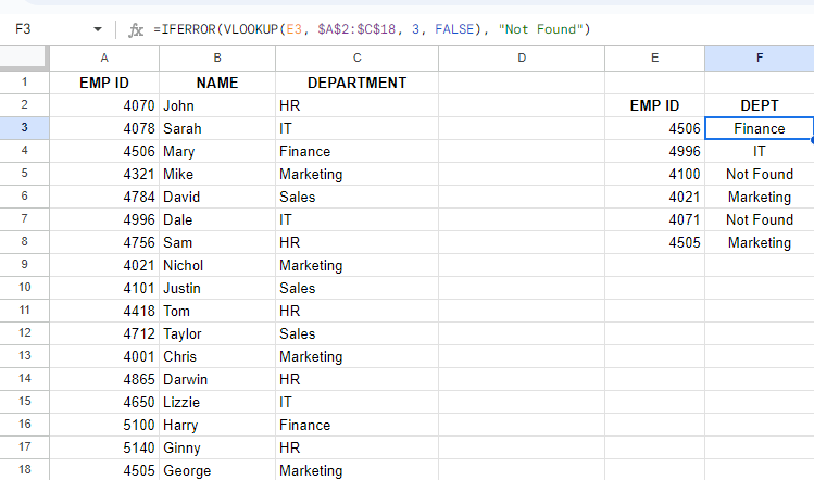
Retrieving the employee's department through ID and handling errors if the employee is not found. Source: Image by Author.

And you can see the results above. Here’s how this formula works: 

• The VLOOKUP(E3, $A$2:$C$18, 3, FALSE) retrieves the employee's department.

• IFERROR handles the errors. Instead of showing an error message (#N/A), it will display a friendly and customized message.

Simply put, you don’t have to dig into sheets anymore. Because when you combine VLOOKUP() and IF() statements, you can tackle even the largest data sets easily in Excel. 

Final Thoughts

By combining VLOOKUP() with IF() statements, you can create more accurate and error-resistant spreadsheets. Make sure to experiment with the examples I shared to see how these techniques can simplify data management tasks and enhance your Excel skills.

If you want to improve your skills, check out our Introduction to Excel course and then upgrade to Excel Fundamentals skill track to master the basics. Once comfortable with these functions, advance your analytical abilities with our Data Analysis in Excel course. But if you’re more on the finance side, check out our Financial Modeling in Excel course to integrate financial insights. 

In addition to this, our Data Preparation in Excel course will help you streamline your data cleaning process, and the Data Visualization in Excel course will help you present your data in a compelling way.