How to Do a VLOOKUP() with Multiple Criteria

VLOOKUP() is one of Excel's most widely-used functions. It allows you to look up and retrieve data from a specific column in a table. In addition to this, it helps merge data from different sheets or find related information.

But did you know that VLOOKUP()’s functionality can be extended to include multiple criteria? This will help users who often need to match multiple conditions when searching for data, which is a common problem that shows up when working with spreadsheets. 

In this article, we’ll see how you can use VLOOKUP() with multiple criteria to level up your work. If you are new to Excel, check out our Introduction to Excel course first to learn the ins and outs of managing tables and applying calculations.

VLOOKUP() Basics

Before we get into VLOOKUP() with multiple criteria, let's first review the basic syntax of VLOOKUP(), which is as follows: 

=VLOOKUP(lookup_value, table_array, col_index_num, [range_lookup])

In the above formula:

• lookup_value is the value you want to search for. This can be a number, text, or a reference to a cell containing the search value.

• table_array is the range of cells that contains the data. The first column in this range should contain the search key.

• col_index_num is the column number in the range from which you want to retrieve the value. 

• range_lookup is where you enter a logical value (TRUE or FALSE). If TRUE, VLOOKUP() assumes that the first column of the range is sorted in ascending order and returns the closest match.

Let's understand this with an example. Here, I have a sheet full of employee-related data, and I want to quickly find a specific employee's name based on their ID number. To do so, I’ll use a VLOOKUP(). 

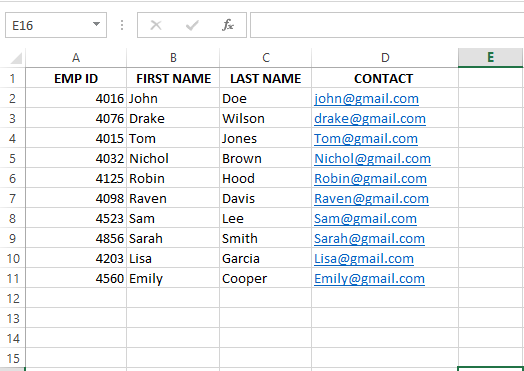
A table containing employee details. Source: Image by Author.

I first enter a value in cell F6 that matches a value in the table. In my case, I'm looking at the EMP ID reference column when I choose 4032.

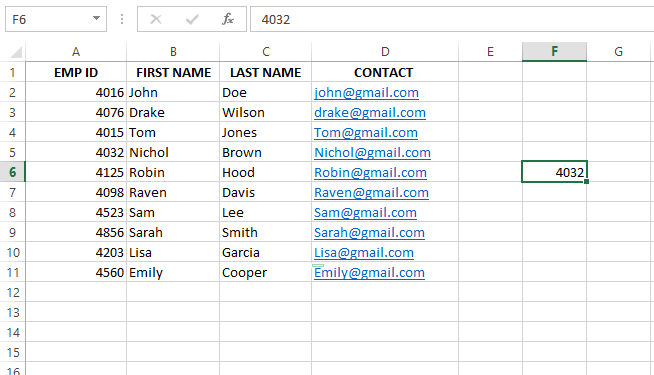
Entering the VLOOKUP() value in a cell. Source: Image by Author.

Then, I select cell G6 and start typing my formula.

Entering VLOOKUP() formula in a cell. Source: Image by Author.

Next, I select the cell where I have entered 4032. This is the value I'm looking up from the table. 

Entering the cell number where the VLOOKUP() value is stored. Source: Image by Author. 

Then, I select the table range (A2:D11). 

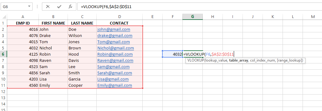
Selecting the range of the table containing data. Source: Image by Author.

Counting from the left, I select column number 2 because I'm looking for FIRST NAME and FIRST NAME is the second column over. 

Entering the column number for which you want results. Source: Image by Author.

After typing FALSE for an exact match, I press Enter. You can see how the VLOOKUP() function finds the employee's FIRST NAME with EMP ID equal to 4032.

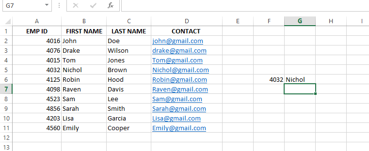
Retrieving the desired output. Source: Image by Author.

How to Use VLOOKUP() with Multiple Criteria

VLOOKUP(), in its basic form, works well for simple lookups, but it can become challenging when you combine multiple criteria. But you can address these limitations with a couple of techniques. Let’s understand how. 

VLOOKUP() with a helper column 

If you need to use a VLOOKUP() with multiple criteria, you can use a helper column to combine multiple criteria into a single criterion. Let's illustrate this with the following example, where I want to find the sales amount for each person based on both a date and a product. 

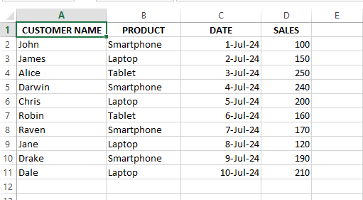
A table containing customer details. Source: Image by Author.

To start with, I create a new column by concatenating the multiple criteria into a unique identifier. In my case, three columns will be concatenated: Customer Name, Product, and Date.

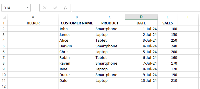
Creating a 'helper' column. Source: Image by Author.

Here is the formula I use to combine the columns into one:

=B2&"|"&C2&"|"&D2

As you can see, there is a pipe symbol after the column name. This works as a separator between each column’s data, and it’s generally considered a good practice when concatenating.

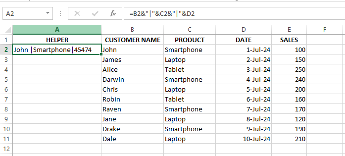
Concatenating three columns in one cell. Source: Image by Author.

If you’re wondering why there is a number instead of a date even though we selected a date column, this is because the date format has been changed to a number format. The lookup will work all the same, but if you want to see the data in a more recognizable form, use the TEXT() function. The TEXT() function takes two parameters: value is the value you want to change, and format_text is the format you want to change the value into.

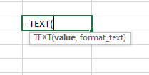
Text formula. Source: Image by Author.

So, to concatenate while also formatting the date, I type the following:

=B2&"|"&C2&"|"&TEXT(D2, "DD-MM-YY")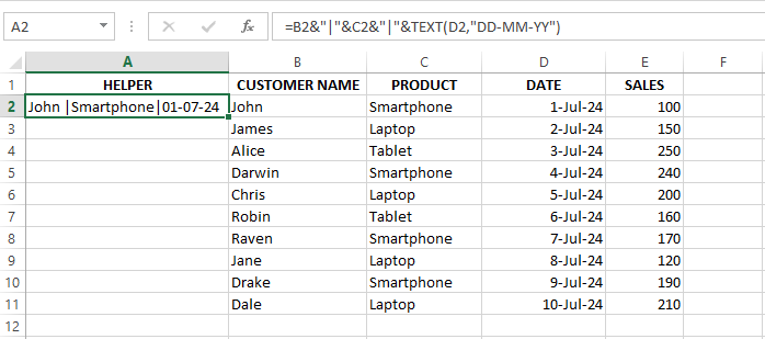

Formatting the date using the TEXT() formula. Source: Image by Author.

Then, I drag the formula down to fill the new column for all rows.

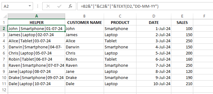
Copying the formula by dragging it. Source: Image by Author.

And you’re done. All three columns are concatenated successfully. Next, I prepare the lookup table, which you can see in the image below. 

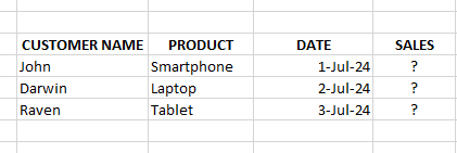
Preparing my table. Source: Image by Author.

Then, I type the following formula and hit Enter. You can see the results below. 

=VLOOKUP(G6&"|"&H6&"|"&TEXT(I6, "DD-MM-YY"),$A$2:$E$11, 5,0)

Retrieving the sales using Vlookup with multiple criteria. Source: Image by Author.

VLOOKUP() with the CHOOSE() function 

The CHOOSE() function selects and returns a value from a list based on a specified index or position. This is the syntax of the CHOOSE() function:

CHOOSE(index_num, value1, [value2], ...)

In this formula:

• index_num is a number that specifies which value to choose.

• value1, value2, … is the list of values to choose from.

The CHOOSE() function can help when you need to look up values based on multiple criteria or when the data structure doesn't fit neatly into a single table. In such cases, CHOOSE() will create a virtual table to combine columns from different sources or reorder columns to match your lookup needs. Let's understand this with an example. I have the following dataset: 

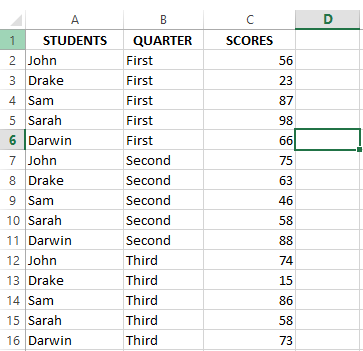
A table containing students' scores in three quarters. Source: Image by Author.

Now, I want to fetch the student’s scores for the first quarter. So, I enter the following formula in cell F2:

=VLOOKUP($E2&"|"&F$1, CHOOSE({1,2}, $A$2:$A$16&"|"&$B$2:$B$16, C2:C15), 2, FALSE)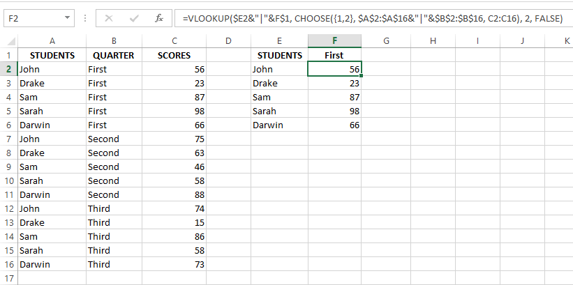

Fetch the scores of students from the first quarter. Source: Image by Author.

Here’s how the formula works:

• CHOOSE({1,2}, $A$2:$A$16&"|"&$B$2:$B$16, C2:C15) creates a virtual helper column by merging multiple criteria into unique identifiers. 

• =VLOOKUP($E2&"|"&F$1, ..., 2, FALSE) searches for the specified value in this virtual first column and retrieves the associated score from the second column.

This way, you can also find what you need without making extra columns on your worksheet.

An Alternative to VLOOKUP() with Multiple Criteria

Although VLOOKUP() is a widely-used function in Excel, it's not the only function for looking up data. You can explore alternatives such as INDEX() and MATCH(). Let’s see how they work together to serve the same purpose of VLOOKUP() with multiple criteria.

INDEX() and MATCH() as VLOOKUP()

The INDEX() and MATCH() functions used together allow for dynamic column lookups. You can use them to work with data not sorted in ascending order, and they can handle horizontal and vertical searches, too. Let’s show this with the following dataset:

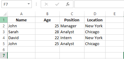
A table containing employee data. Source: Image by Author.

From this data, I want to find the position of John, who is 25 and lives in Chicago. 

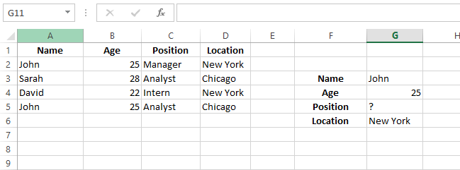
Creating a reference table. Source: Image by Author.

Now we type the following formula in G5:

=INDEX(C2:C5,MATCH(1,(G3=A2:A5)*(G4=B2:B5)*(G6=D2:D5),0))

Using INDEX() and MATCH() together. Source: Image by Author.

Final Thoughts

I've covered some of the most important techniques that can be used with VLOOKUP()—helper columns, array formulas, and even fancy functions like INDEX() and MATCH(). These methods make it easier to handle large datasets and make you more confident in your data.

If you want to learn more about data analysis and visualization in Excel, check out these courses: Data Analysis in Excel and Data Visualization in Excel. We also have a shorter read, which is our Visualizing Data in Excel tutorial.