Rank Formula in Excel: A Comprehensive Guide With Examples

Ranking lets you compare values and identify patterns within your datasets. Excel provides powerful tools such as RANK(), RANK.EQ(), and RANK.AVG() to make ranking easier. These functions are helpful in all situations, from ranking participants in a sports tournament by points to analyzing market trends based on ranked sales data.

In this article, we’ll explore all three rank functions in Excel and explain how you can use them with hands-on examples. We will also dive into using rank functions with other Excel functions and calculating percentile ranks. 

The Quick Answer: How to Calculate Rank in Excel 

To calculate the ranks in your desired datasets, use the following formula:

=RANK(number, ref, [order])

Understanding the RANK() Function in Excel

Let’s say you organized a competition among school students and now want to rank thousands of students based on their performance. 

Would you spend hours sorting through data? No, because Excel can help. Among its many powerful functions is the RANK() function, which lets you determine someone's position with a single click. 

To calculate the rank of a value within a range of values, enter the formula:

RANK(number, ref, [order])

In the above formula:

• number: is the number you want to rank.
• ref: is the range of numbers to take into account for ranking.
• order: specifies the rank order. For ascending, use “1” as a value; for descending, use “0” (default).

How to Use the RANK() Formula in Excel

Let’s implement the RANK() function on real-world examples:

Ranking students grades

Calculating grades would be challenging and time-consuming if you have thousands of students. Suppose you're preparing final results for students and want to rank them based on scores. 

To do so, first, prepare your dataset.

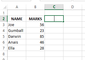
Students example dataset in Excel. Source: Image by author.

Enter the formula =RANK(B3,($B$3:$B$7)) in one cell and drag it to the last filled cell to get the rank.

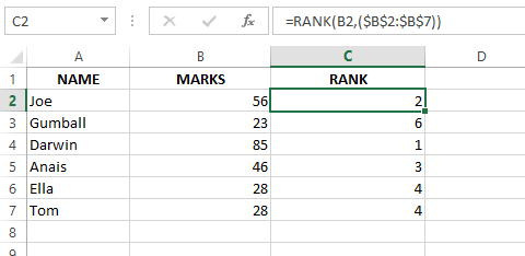
Using the RANK() function to calculate the rank of students. Source: Image by author.

You now have the student’s rank in just one click.

But did you notice that two students with the same marks have the same rank of 4? The following student, with 23 points, jumps to rank 6, skipping rank 5. This means that the formula assigns the same rank to duplicate scores. 

This can mess up the order for close scores. But you can fix these ties using the COUNTIF() function. Enter the following formula: 

=RANK(B3,($B$3:$B$8)) + COUNTIF($B$3:B3, B3)-1

The COUNTIF() function adjusts the rank for duplicate values. It counts how many times the current student's marks appear above them in the list.

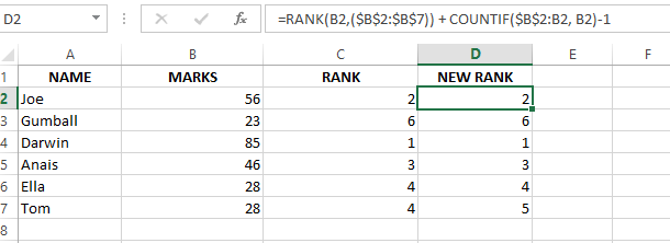
Breaking ties using the COUNTIF() function in Excel. Source: Image by author.

A value of 28 appears twice, and COUNTIF() tracks the occurrence count. This occurrence count is used to adjust the rank. The formula adds the count of occurrences minus one to the original rank. This ensures that each duplicate value receives a unique rank.

Ranking sales figures in a dataset

Let’s look at another example to show how to use the Excel RANK() function in ascending or descending order. 

If you want to assess your sales team's performance, you can rank their monthly sales figures using Excel's RANK() function.

Here, we have a dataset with monthly sales figures for each salesperson. We'll use the RANK() function to rank them based on who brought in the most sales (highest to lowest).

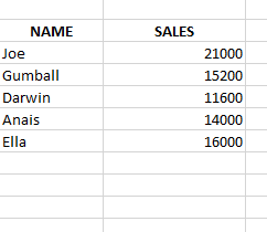
List of sales figures to rank. Source: Image by author.

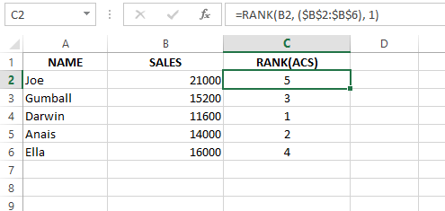
To rank the sales in ascending order, we applied the formula =RANK(B2, ($B$2:$B$6), 1). Here, a value of “1” for the order parameter specifies the ascending order for the ranking. 

Ranking the values in ascending order. Source: Image by author.

Once you've entered the formula, simply hold the cursor, drag the corner of the cell down, and apply it to the rest of your sales data.

Similarly, if you want to rank the values in descending order, write “0” as the order parameter value in the formula like this: =RANK(B2, ($B$2:$B$6), 0)

You can see the difference in the results:

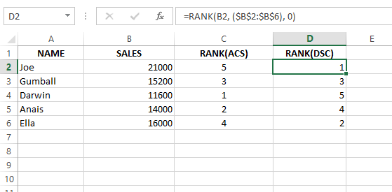
Ranking the values in descending order. Source: Image by author.

You may notice the dollar signs in the references ($B$2:$B$6). These are called absolute references. They ensure the formula always refers to the same sales data range, even when you copy it down, to prevent errors.

If you don’t use the absolute reference, like =RANK(A2, A2:A10), the range will adjust as you drag down:

• Formula in G3: =RANK(G3,(G3:G7), 1)
• Formula in G4: =RANK(G4,(G4:G8), 1)

To prevent this issue, use absolute references by pressing “F4”. Now the formula will be: =RANK(G3,($G$3:$G$7), 1)

When you drag the above formula to the last filled cell, relative references will change based on each cell's position. You can see the difference in the results when using absolute references:

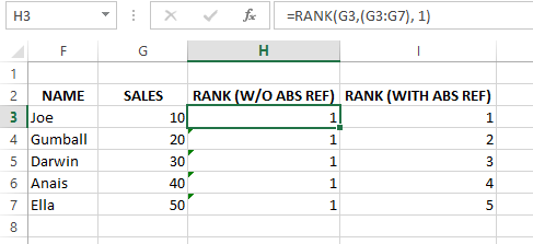
Difference between the ranks with and without absolute reference. Source: Image by author.

Advanced Rank Excel Functions: RANK.EQ() and RANK.AVG()

When you encounter duplicate values in Excel, things can get tricky. That's where I prefer using the RANK.EQ() and RANK.AVG() functions. Both of them are slightly different to handle. Let’s look at how they work.

The RANK.EQ() Excel function

RANK.EQ() works just like the regular RANK() function but with a more precise name. When there are duplicates, RANK.EQ() assigns the same rank to all of them and simply skips the next rank(s) in line.

Syntax: =RANK.EQ(number, ref, [order])

In the above formula:

• number: is the number you want to rank.
• ref: is the range of numbers to take into account for ranking.
• order: specifies the rank order. For ascending, use “1” as a value; for descending, use “0” (default).

Let’s understand this formula with an example: I had a dataset with the populations of several countries, and I  wanted to rank these countries based on their populations.

Here's how I did it using the RANK.EQ() function:

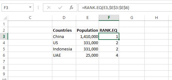
Using the RANK.EQ() function. Source: Image by author.

In the image above, the country with the highest population is ranked 1, and so on. Now, you see how RANK.EQ() handles ties. 

Since the US and Indonesia have identical populations, they share the same rank of 2. This makes it clear how RANK.EQ() assigns the same rank to duplicates and skips the next rank in the sequence.

The RANK.AVG() Excel function

The RANK.AVG() function takes a different approach to handling ties in rankings. Instead of assigning the same rank to all duplicates, it calculates the average of the ranks they would have received individually.

Syntax: RANK.AVG(number, ref, [order])

In the above formula:

• number: is the number you want to rank.
• ref: is the range of numbers to take into account for ranking.
• order: specifies the rank order. For ascending, use “1” as a value; for descending, use “0” (default).

Let’s understand this with an example: I had a dataset of scores, so I applied the RANK.AVG() function to see how it handles tie scores.

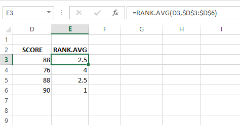
Using the RANK.AVG() function. Source: Image by author.

Using =RANK.AVG(D3,$D$3:$D$6), the score 88, receives a rank of 2.5. This means the function averages the ranks it would have assigned individually. 

This approach maintains a more balanced distribution of ranks, especially in datasets with frequent ties.

Combining RANK() With Other Excel Functions

Using the RANK() function with other Excel functions is helpful in some scenarios. Let’s review a couple of common use cases.

Combining RANK() and ROUNDUP() to categorize data

Here’s how you can combine the ROUNDUP() function with the RANK() function:

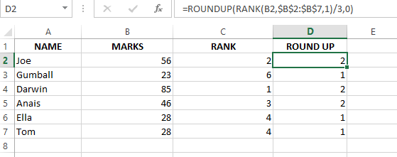
Combining the RANK() and ROUNDUP() functions in Excel. Source. Image by author.

I used the formula =ROUNDUP(RANK(B2, $B$2:$B$7, 1)/3, 0), which calculates the rank of the value in cell B2 within the range B2 in ascending order. It then divides this rank by three and rounds up the result to the nearest integer.

With the above formula, you effectively categorize the data into distinct groups or tiers, which can help identify and analyze different performance levels or categorize data for further analysis.

Combining RANK.EQ() and COUNTIFS() to break ties

We have discussed a few ways to handle ties using Excel's RANK() function. However, let’s say you want to rank products solely based on price. This might feel arbitrary when multiple items share the same cost. 

So, let's introduce a secondary criterion to break ties and create a more objective ranking system.

Consider a list of customers who have bought headphones. We want to rank them by their price (primary criteria) and then use customer rating (secondary criteria) to differentiate in case of a tie.

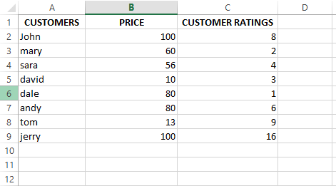
Example list of customers. Source: Image by author 

To achieve this, we'll combine the RANK.EQ() function with the COUNTIFS() function. Here’s how:

=RANK.EQ($B2,$B$2:$B$9) + COUNTIFS($B$2:$B$9, $B2, $C$2:$C$9, ">"& $C2)

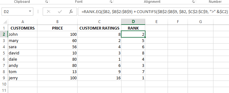Calculating rank using RANK.EQ() and COUNTIFS(). Source: Image by author.

The section COUNTIFS($B$2:$B$9,$B2)counts how often the current price appears in the list. We use absolute references for the range, $B$2:$B$9, to maintain consistency but keep the criteria cell, $B2, relative so the formula checks each row individually.

The second part, $C$2:$C$9,">"&$C2, finds the number of customer ratings higher than the current headphone's rating, C2.

COUNTIFS() follows “AND” logic: It only counts cells that meet all conditions. If no other headphones at the same price have a higher rating, COUNTIFS() returns 0. That’s why the rank determined by RANK.EQ() remains unchanged.

Calculating Percentile Rank in Excel

Since the RANK() function ranks a numeric value, you can use an Excel percentile rank formula to calculate the value rank within a dataset as a percentage of the total dataset. 

Excel provides two functions for calculating percentile ranks. Let’s explore both of them. 

The PERCENTRANK.INC() Excel function

PERCENTRANK.INC() calculates a value's percentile rank, including the smallest and largest values in the dataset.

Let’s understand this function with an example: I had a dataset representing the exam scores of 10 students, and I wanted to calculate the percentile rank of each score, including the smallest and largest values. 

So, I used the formula =PERCENTRANK.INC($A$2:$A$11, A2):

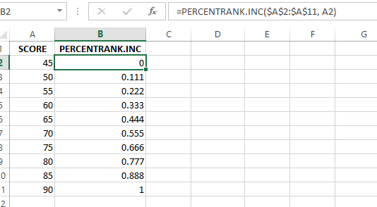
Calculating the rank using the PERCENTRANK.INC() function. Source: Image by author

In the above example, you can see the PERCENTRANK.INC() function includes the smallest and largest values in the dataset. The score 45 (smallest value) has a percentile rank of 0, and the 90 (largest value) score has a percentile rank of 1.

The PERCENTRANK.EXC() Excel function

PERCENTRANK.EXC() calculates a value's percentile rank, excluding the smallest and largest values in the dataset.

Let’s understand this function with an example:  I applied the PERCENTRANK.EXC() function on the same student dataset from the previous section:

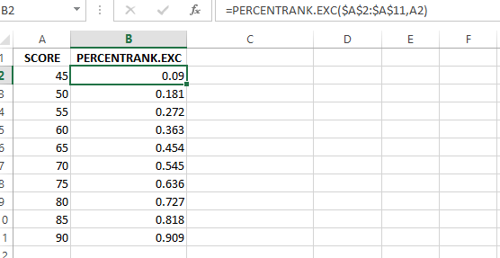
Calculating the rank using the PERCENTRANK.EXC() function. Source: Image by author

In the above example, the PERCENTRANK.EXC() function excludes the smallest and largest values in the dataset. This means the score 45 (smallest value) does not have a percentile rank of 0, and the score 90 (largest value) does not have a percentile rank 1.

Excel RANK() Function Common Mistakes and How to Avoid Them

Excel functions are handy and easy to use for all business work. But sometimes, even the most skilled users can make a few common mistakes. So, I’m sharing some of the most common mistakes to look for and how you can avoid them:

Copy-pasting formulas

When you copy your ranking formula across cells, make sure you don't accidentally use absolute references. Each cell can reference a different chunk of data and disrupt your rankings. 

To avoid this, use absolute references, like $A$1:$A$10, when setting up your formulas to lock in the correct range across all your rankings.

Not handling duplicates

Let's say you have two salespeople tied for the most sales. How you handle ties in your ranking can make a big difference: the RANK() and RANK.EQ() functions treat ties similarly.

So, you should decide if tied values deserve the same or different rank or if their ranks should be averaged using RANK.AVG(). Then, use the correct function accordingly. 

Wrong ordering 

It seems simple, but forgetting to set the order argument in your function can sort rankings in the wrong direction (ascending or descending). 

That’s why you should always double-check this argument: Use “0” (or leave it blank) for descending order and “1” for ascending order. Make sure the order aligns with how you want your data ranked.

Function fumble

When you work with different datasets, it’s so important to choose the correct rank function because proceeding with the wrong ranking function will give undesirable results.

To avoid these issues, use RANK.EQ() for standard ranking and RANK.AVG() for scenarios where tie handling affects the outcome, like statistical analysis. 

Using outdated formulas 

As your data grows, you must update the range references in your formulas. This means new data points won't be included in your rankings, and you may get frustrated about why you are not getting your answer right.

That’s why you should regularly update and check the ranges in your formulas. This ensures that all your valuable data is considered for ranking.

Final Thoughts

Now you know how to use functions like RANK(), RANK.EQ(), and RANK.AVG() to handle ties and solve various ranking problems. These functions help in different scenarios, such as analyzing student grades or ordering sales figures.

If you’re interested in expanding your Excel skills further, I highly recommend checking out some excellent courses and resources available on Datacamp: 

• Start with the Introduction to Excel course to build foundational knowledge, then advance to Data Analysis in Excel and Excel Fundamentals.  
• Consider the Data Visualization in Excel course to enhance your ability to visualize data. 
• The Introduction to PowerQuery in Excel course greatly benefits more advanced data manipulation. 
• However, to formalize your Excel expertise, check out this comprehensive guide on How to Earn a Microsoft Excel Certification.