How to Remove Duplicates in Excel: 5 Best Methods

Method 1: Remove duplicates with Conditional Formatting

You can use the Conditional Formatting feature to highlight duplicates or unique values and decide whether to remove them. To do so:

• Select the range of cells you want to check. Then, go to Home > Conditional Formatting > Highlight Cells Rules > Duplicate Values.

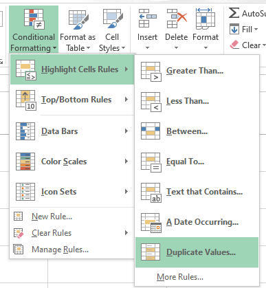
Select the Duplicate Values option. Image by Author.

• A dialog box appears. From the drop-down list, select how you want to highlight the duplicates. Here, I chose Yellow Fill with Dark Yellow Text.

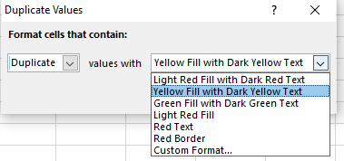
Apply the format. Image by Author.

• Click OK and see the duplicate values highlighted. 

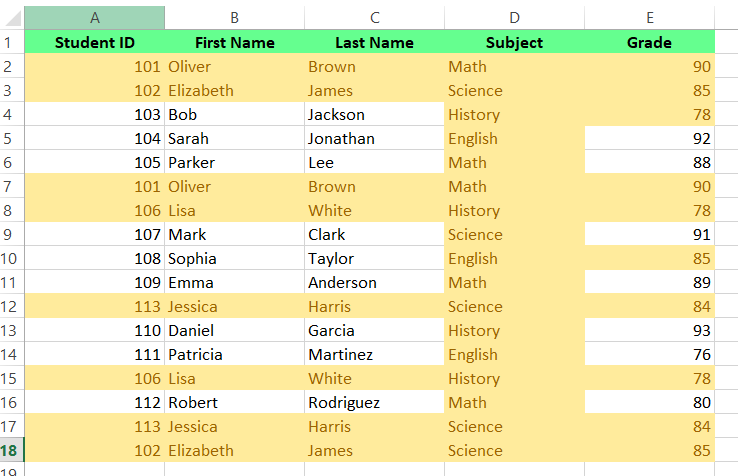
Duplicate values are highlighted. Image by Author.

However, the Conditional Formatting feature is limited — it can't highlight duplicate values within the Values area of a PivotTable report. In that case, you have to use a different method. 

Method 2: Use the Remove Duplicates feature

Another quick way to remove duplicates is to use the Remove Duplicates feature, a built-in Excel tool that cleans up your data by removing duplicates permanently. To use this method:

• Select the range of cells or click on a cell, and Excel will automatically identify the range of cells.

Identifying the range of cells. Image by Author.

• Next, go to the Data tab  > Data Tools and select Remove Duplicates.

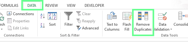
Remove Duplicates feature. Image by Author.

• A dialog box will appear. Here, I select the columns that should be checked for duplicates. If your data includes column headers, check the My data has headers box and click OK.

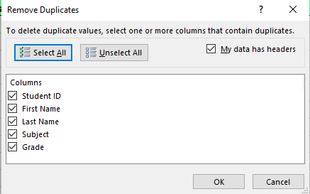
Dialog box for the Remove Duplicates feature. Image by Author.

• Excel will display a message showing the number of duplicates removed and the number of unique entries remaining.

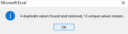
Message box. Image by Author.

• Now you can see all the duplicate rows are removed.

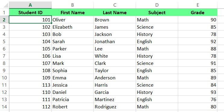
Removed all the duplicate rows. Image by Author.

Method 3: Remove duplicate values using the Advanced Filter option

You can also use the Advanced Filter function in Excel to extract unique values by filtering out duplicates, keeping the original data while showing unique entries. Here's how you can use it:

• Select a range of cells or a single cell and Advanced Filter will automatically identify the range. Next, go to the Data tab > Sort & Filter and click Advanced.

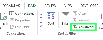
Advanced feature option. Image by Author.

• A dialog box will appear. To copy unique values to a different location, select Copy to another location. In the Copy to field, specify where to display the unique values. Then, select the Unique records only box and click OK.

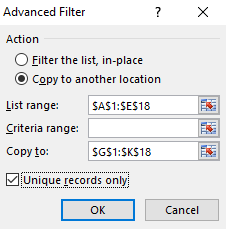
Dialog box for the Advanced Filter. Image by Author.

• Now, all the unique values are copied to our specified range.

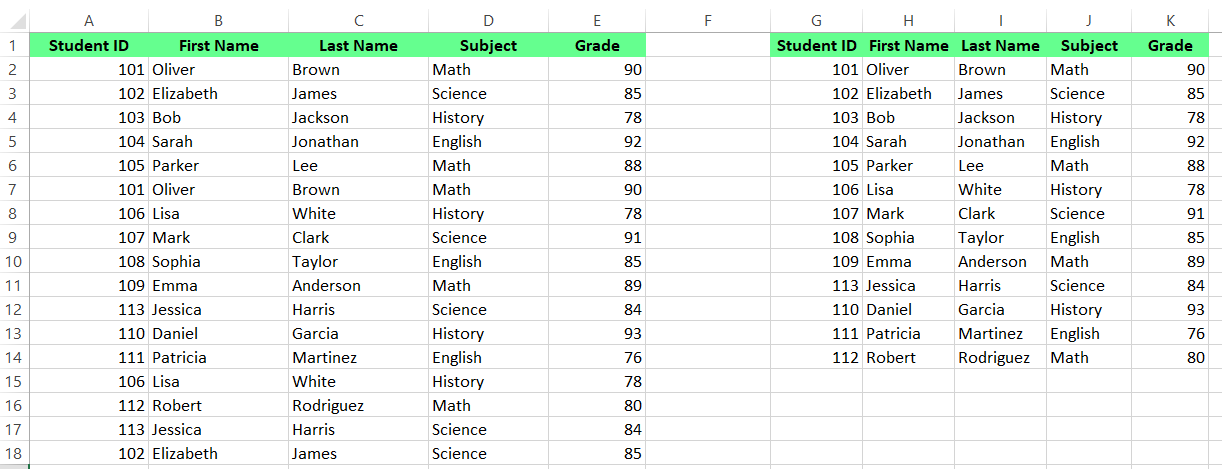
Filter the unique values using Advanced Filter. Image by Author.

Method 4: Remove duplicates with formulas

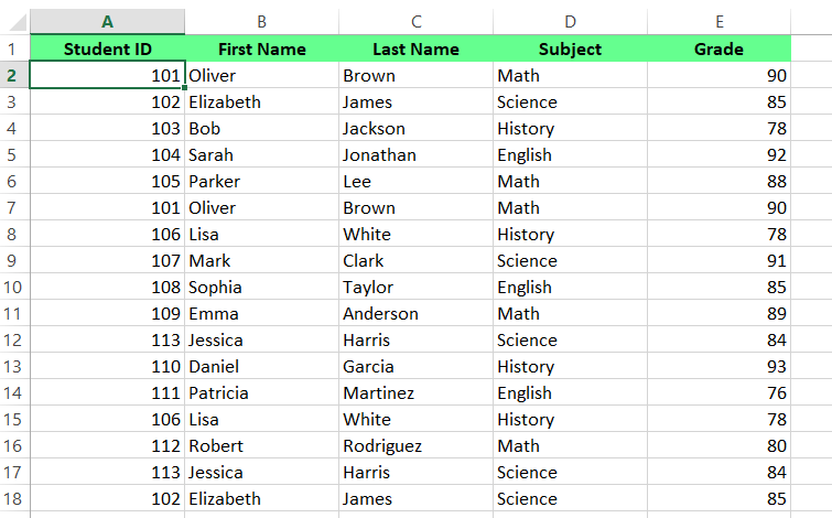
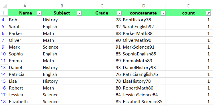
Now that you know 3 built-in features for removing duplicates, let's understand some custom functions you can create to achieve the same result. For example, I have a dataset with Name, Subject, and Grade columns.

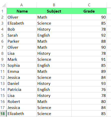
Dataset of students. Image by Author.

To create a formula for filtering out duplicate values:

First, I combine all the columns (A,B,C) in one cell. There are two methods to do this: the CONCATENATE() function or the & operator. Choose whatever you like and the results will be the same. To use & operator, type the following formula: 

=A2&B2&C2

 To use CONCATENATE() function, type the following formula: 

=CONCATENATE(A2,B2,C2)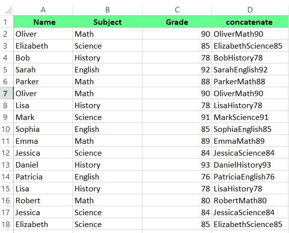

Concatenate the columns. Image by Author.

In the next column, use COUNTIF() to calculate the number of times each value appears in column D:

=COUNTIF(D2:D18,D2)

Here, count 1 means the value is unique, and count  2 or more indicates a duplicate.

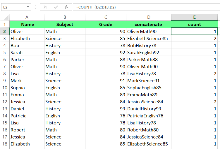
Apply COUNTIF() to count the occurrences. Image by Author.

Next, go to Data tab > Sort & Filter > select Filter to apply a filter to the count column. 

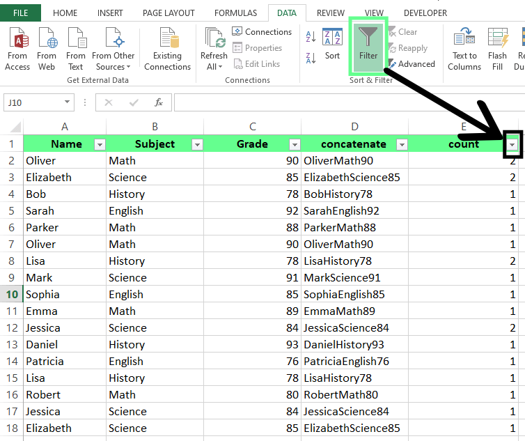
Apply Filter. Image by Author.

Then, open the drop-down menu, select 1 to keep unique values and eliminate duplicates, and hit OK.

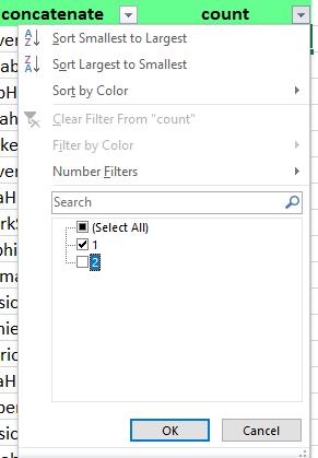
Keep the unique values. Image by Author.

Now you can see all the duplicate values have been removed. This method is more complex but dynamically updates as your data changes, so it’s perfect for those who want ongoing duplicate management.

Duplicate values removed using the Filter feature. Image by Author.

Method 5: Remove duplicates using Power Query

You can also use Power Query to clean your data and remove duplicates. Here’s how:

Select a cell or range of cells. Go to the Data tab > Get & Transform Data section and click From Table/Range. A dialog box will appear to create a power query table, and the range of values will be automatically selected. Then hit OK.

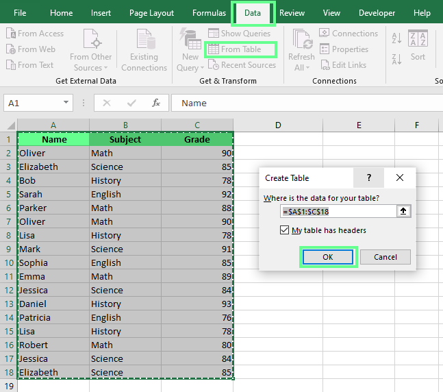
Creating a table. Image by Author.

Now, the Power Query editor window will appear. From there, choose the Remove Duplicates option to select specific columns or the entire table. For the whole table, click on the top left corner button. For a specific column, right-click on the particular header or use CTRL to select more than one column. Once done, click the Close & Load option at the top left corner to load the cleaned data back into Excel.

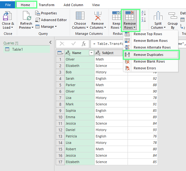
Removing duplicate data. Image by Author.

You can see the modified dataset appears back in Excel. To understand this further, you can select another column, like Subject, from this example, and repeat the steps for practice. This way, only those rows where the student name is duplicated will be removed.

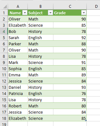
Data loaded in an Excel sheet. Image by Author.

This method is perfect if you work with large datasets or need to automate the duplicate removal process for future data refreshes. 

Methods to Remove Duplicates in Excel: Which One’s The Best?

We've seen five different methods to remove duplicates in Excel. Now, I want to help you choose which one is best, but before I do, let's first talk quickly about the two types of duplicate data. 

Different types of duplicate data

So far, to be clear, I've focused on how to remove duplicate values in a column, and every method I have shown so far works if this is your issue. However, to be clear, in Excel, duplicates can appear in two forms — duplicate values and duplicate rows:

• Duplicate values are repeated entries in a single column. For example, if I have a column of names and Minny appears multiple times, those are duplicate values.
• Duplicate rows occur when entire rows have identical data across all columns. For example, my table has Name, Age, and City columns. If two or more rows have the same fields, they are duplicate rows.

Summary table

Here's a summary table that shows the specific advantages of each method. Here, I've also added a column to show if the method can be extended to remove duplicate rows as well. Basically, if you want to remove an entire duplicate row, try Conditional Formatting, Advanced Filter, Formulas, or Power Query, but leave the Remove Duplicates Features for simple use cases.

Here are a couple of best practices I recommend when starting any data cleanup project:

• Keep Backup: Always maintain an untouched backup of your raw data before starting any cleanup. You can use the original version as your reference point whenever needed.
• Define your Duplicates: Establish clear criteria for what constitutes a duplicate in your specific context. Sometimes, it's not as simple as exact matches across all fields.
• Standardize First: Clean and standardize your data before attempting duplicate detection — normalize case, trim spaces, fix date formats, and handle special characters.
• Start Simple, Then Refine: Begin with exact matches before moving to more complex matching. This approach will help you incrementally understand your data quality.
• Validate Your Results: Spot-check your results when using automated tools to catch systematic errors.

Troubleshoot Common Excel Issues

Let’s look at the most common problems that you may come across when removing duplicates.

Duplicates not removed

Sometimes, we copy data from websites or external sources — this data usually contains hidden characters or spaces that prevent Excel from identifying duplicate entries. To solve this issue, you can use the TRIM() and CLEAN() functions. The TRIM() function will remove excessive spaces between words, and the CLEAN() function will remove non-printable characters.

=CLEAN(TRIM(A1))

Data with subtotals or outlines

If your spreadsheet contains subtotals or outlines, they can interfere with the duplicate removal process. Excel treats these summary rows as unique entries, which can lead to incomplete duplicate removal. To avoid this, remove all subtotals and outlines from your data before removing duplicates. 

Here’s how you can do so:

• To remove outlines: Go to the Data tab, find the Outline group, and click Clear Outline.
• To remove subtotals: Go to the Data tab, click Subtotal, then click Remove All.

After removing outlines and subtotals, you can proceed with duplicate removal as usual.

Case sensitivity

Excel considers uppercase and lowercase text as different values when checking for duplicates. For example, Product and PRODUCT would be treated as different entries. To avoid this, use the UPPER(), LOWER() or PROPER() functions to standardize the text case across all your data before starting the removal process.

• =UPPER() convert text to uppercase. 

• =LOWER() converts text to lowercase. 

• =PROPER() capitalizes the first letter of each word.

Final Thoughts

Cleaning up duplicates in Excel may seem like a small task, but it can make a big difference in your work. I've covered five ways to do this, from quick built-in features to more advanced techniques. You should try different methods until you find an approach that fits smoothly into your workflow and keeps your data accurate. 

If you want to strengthen your Excel skills further, check out our Data Analysis in Excel course and Data Analysis with Excel Power Tools skills track.