How to Highlight Duplicates in Excel

Method 1: Highlight duplicates in Excel using conditional formatting

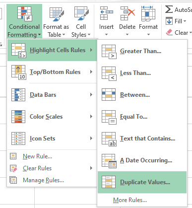
You can use conditional formatting to identify duplicates in your Excel spreadsheet. Here’s how:

• Select the range of cells you want to check.

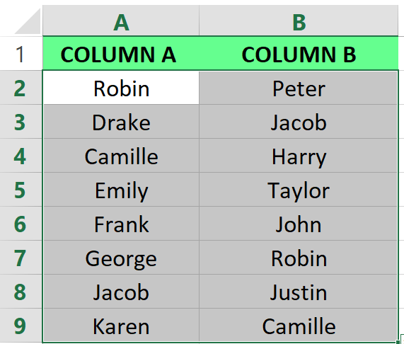
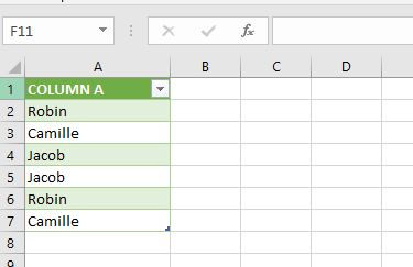
Select the range of cells. Image by Author.

• Go to Home > Conditional Formatting > Highlight Ccells Rules > Duplicate Values.

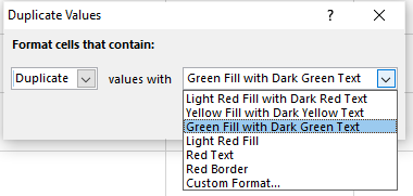
Select the Duplicate Values option. Image by Author.

• A dialog box appears. From the drop-down list, select how you want to highlight the duplicates. Here, I chose Green Fill with Dark Green Text.

Apply the format. Image by Author.

• Click OK and see the duplicate values highlighted.  

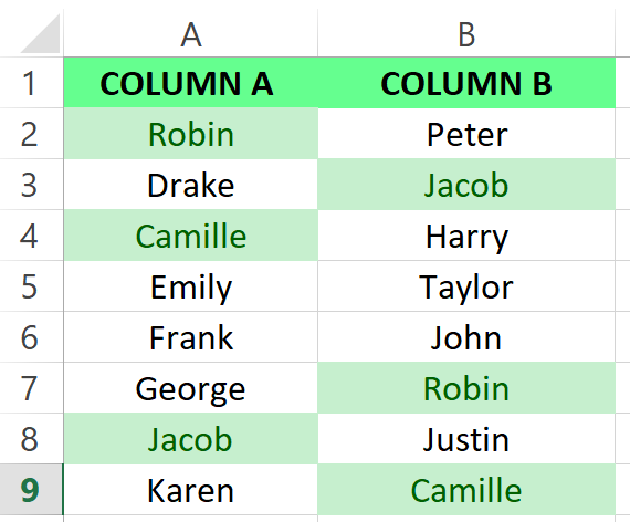
Duplicate values are highlighted. Image by Author.

The best thing about this approach is that you can see duplicates right away. As soon as you enter new data, Excel will automatically color it if it's a duplicate. While this method is quick and easy, it has some basic limits. For example, if you want to check for duplicates across multiple columns or find partial matches (like just matching last names), this simple highlighting won't work. 

Method 2: Highlight duplicates in Excel using the COUNTIF() formula

Here’s how you can highlight only the second and subsequent duplicate values. As a note, this method won't count the first occurrence.

• Select the range of cells. 
• Go to the Home tab > Conditional Formatting > New Rule.

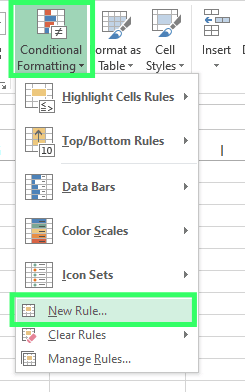
Setting a new rule. Image by Author.

• Now, select the Use a formula to determine which cells to format option. Then, in the formula box, type the following formula. (Here, A2 is the first cell in the range you selected.)

=COUNTIF($A$2:$A2,$A2)>1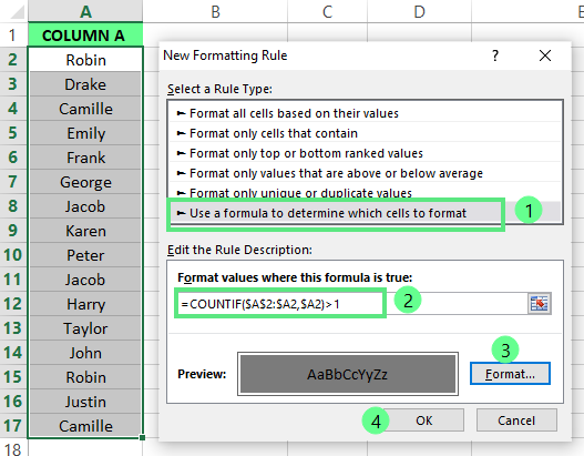

• Click the Format button to choose your desired fill or font color, then select OK to apply changes.

Steps to highlight the duplicates. Image by Author.

Now you can see all the duplicate cells are highlighted, excluding the first occurrences.

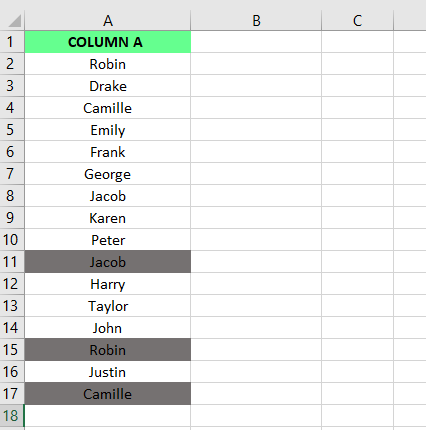
Highlighted duplicates. Image by Author.

Like the Conditional Formatting option, the formula automatically recalculates as your data changes and duplicates are identified in real-time. But here’s how the most outstanding part — you get more control over duplicate data with this method. Suppose you only want to check for duplicates in specific columns, or maybe you want to count something as a duplicate only if both the name AND email match. This method lets you do that by adjusting your formula.

Method 3: Highlight duplicates in Excel with Power Query

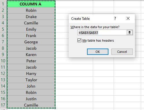
You can use Power Query to import and clean data from multiple sources. It’s especially helpful for handling large datasets and performing more advanced data manipulation tasks. Here’s how you can use it to highlight duplicates:

• Select a cell or range of cells. 
• Go to Data tab > Get & Transform Data > From Table.

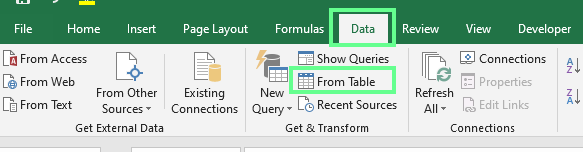
Selecting the From Table option. Image by Author.

• A pop-up will appear. If you have a header in your data, make sure to check the My table has headers option so it doesn't count your header as data. Next, select OK.

Selecting the data automatically. Image by Author. 

• The selected data appears on the Power Query Editor. Now, select the column you want to check for duplicates.

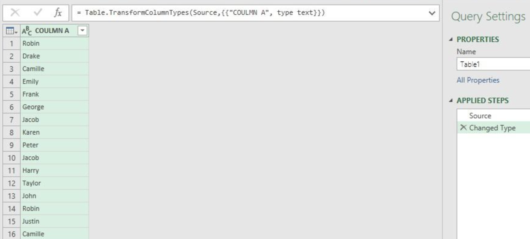
Power Query Editor. Image by Author.

• Next, inside the Power Query Editor, go to the Home tab > Keep Rows and select the Keep Duplicates option. This will display all the duplicate rows of the selected column.

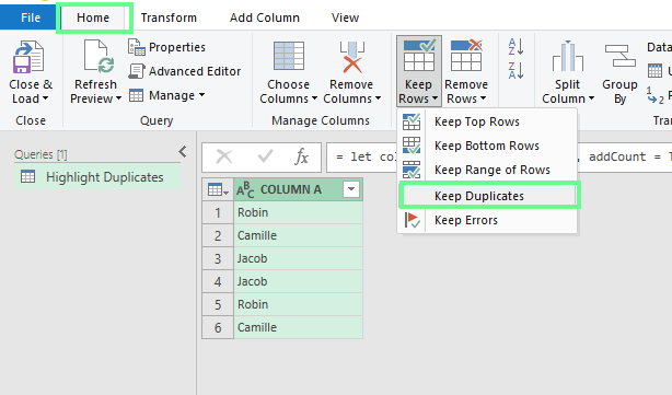
Showing duplicate data. Image by Author.

• If you want to see the results in Excel rather than Power Query Editor, click Close & Load under the Close group. 

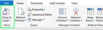
Close & Load. Image by Author.

This way, you can see the results in Excel.

Data loaded in excel sheet. Image by Author.

This approach works well with large datasets — hundreds or even thousands of rows. It's also perfect if you regularly get new data and need to check for duplicates often. Instead of doing the same work repeatedly, you set it up once, and Power Query will automatically clean up any duplicates.

Best Practices for Highlighting Duplicates in Excel

If you want to highlight duplicates in Excel, adopt a systematic approach to maintain the integrity of your data. Here are some of my best practices that you can follow:

• Before making any modifications, always backup your data. This ensures you have a safety net to revert to.
• Standardize all text cases, spaces, dates, numbers, and special characters to maintain consistent formatting.
• Set data validation rules, including dropdown lists, warning messages, required fields, value ranges, and documented procedures to prevent duplicates at the entry point.

Troubleshooting Common Excel Duplicate Issues

Even with the right methods, you can encounter a couple of challenges while highlighting duplicates. While the following functions aren't necessary for you to find duplicates per se, knowing them can help you fix common issues.

Duplicates not highlighted

Sometimes, values with identical names aren't highlighted due to hidden characters or extra spaces. To solve this issue, use the TRIM() and CLEAN() functions together. TRIM() will remove unnecessary spaces from the text's beginning, end, and middle, while CLEAN() will eliminate non-printable characters. 

Case sensitivity

Excel is case-sensitive. It treats uppercase and lowercase letters as different characters, such as DATACAMP, DataCamp, Datacamp, and datacamp, which would be considered different entries. To solve this, you can use the UPPER(), LOWER() and PROPER() functions. Here’s what each function does:

• UPPER() converts text to uppercase. 

• LOWER() converts text to lowercase.

• PROPER() capitalizes the first letter of each word.

Final Thoughts

Regular duplicate checks maintain data integrity and prevent analysis errors. While Excel has several approaches to highlighting duplicates, I encourage you to experiment with different methods to find what best suits your needs.

If you want to strengthen your data handling expertise further, check out our Data Analysis in Excel course and Data Analysis with Excel Power Tools skill track.