SUBTOTAL() Formula in Excel: A Full Calculation Guide

Excel users often need flexible ways to summarize data that respond to filters or groupings. Traditional functions like SUM(), AVERAGE(), or COUNT() calculate results based on all cells in a range, regardless of whether some rows are hidden or filtered out. The SUBTOTAL() function offers a dynamic alternative that automatically adjusts its calculations based on what's currently visible in your worksheet.

If you're new to Excel and want to build a solid foundation before exploring advanced functions like SUBTOTAL(), our Introduction to Excel course covers essential skills including worksheet navigation, basic formulas, and data formatting techniques that will prepare you for more sophisticated Excel work.

What Is the SUBTOTAL() Function in Excel?

The SUBTOTAL() function calculates aggregate values such as sum, average, count, and other statistical operations on a dataset. What makes it different from standard Excel functions is how it works dynamically—changing its result based on what's visible or filtered. The function can ignore both manually hidden rows and rows hidden through filters, depending on which function number you specify.

When you apply a filter to your data or manually hide certain rows, SUBTOTAL() automatically adjusts its calculation to include only the visible cells. This behavior makes it an excellent choice for creating summary rows in filtered datasets, building interactive dashboards, or generating reports that need to update based on user selections.

The function supports the same statistical operations as Excel's standard functions—including sum, average, count, maximum, minimum, and several others—but packages them into a single, context-aware function that adapts to your data's current state.

Syntax and Supported Operations

The SUBTOTAL() function follows a straightforward syntax structure:

=SUBTOTAL(function_num, ref1, [ref2], ...)

The first parameter, function_num determines both the type of calculation and how the function handles hidden rows. The remaining parameters (ref1, ref2, etc.) are the cell ranges you want to include in the calculation. You can specify up to 254 different ranges.

The function numbers fall into two distinct categories based on how they treat manually hidden rows:

Function numbers 1-11 include cells from manually hidden rows in their calculations, while function numbers 101-111 exclude them. However, both ranges always ignore rows hidden by filters.

For example, SUBTOTAL(9, A2:A10) calculates the sum of A2:A10 including any manually hidden rows, while SUBTOTAL(109, A2:A10) excludes manually hidden rows from the sum calculation. In both cases, filtered rows are automatically excluded from the result.

SUBTOTAL() Function Example in Action

Let's see how SUBTOTAL() works with a practical example using sales data from an electronics and furniture store.

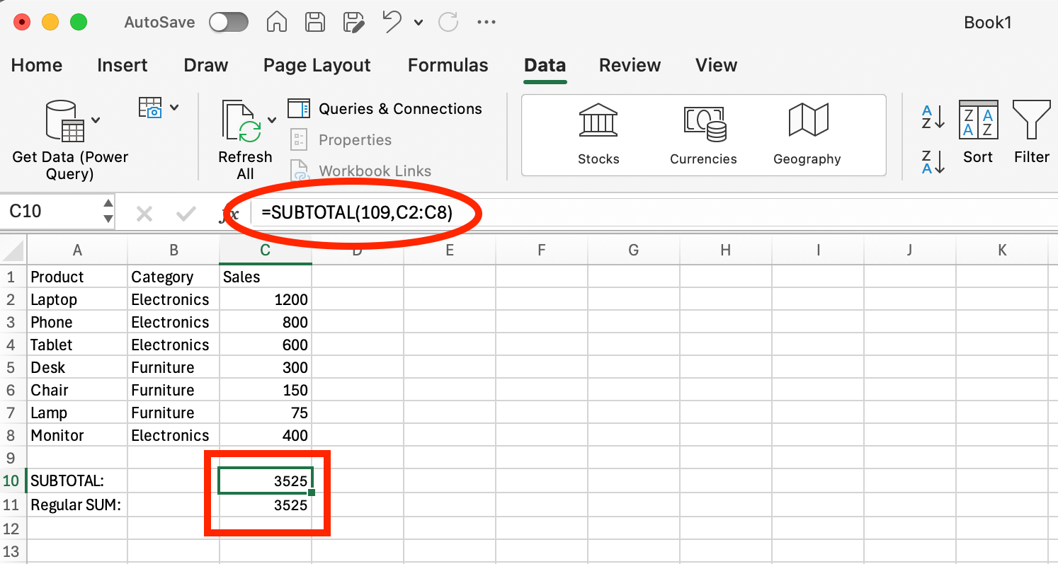
Unfiltered Dataset. Image by Author. 

Our sample data contains seven products across two categories - four Electronics items (Laptop, Phone, Tablet, Monitor) and three Furniture items (Desk, Chair, Lamp). With no filters applied, both the SUBTOTAL(109,C2:C8) formula and regular SUM(C2:C8) formula show the same result: 3525 (the total of all sales).

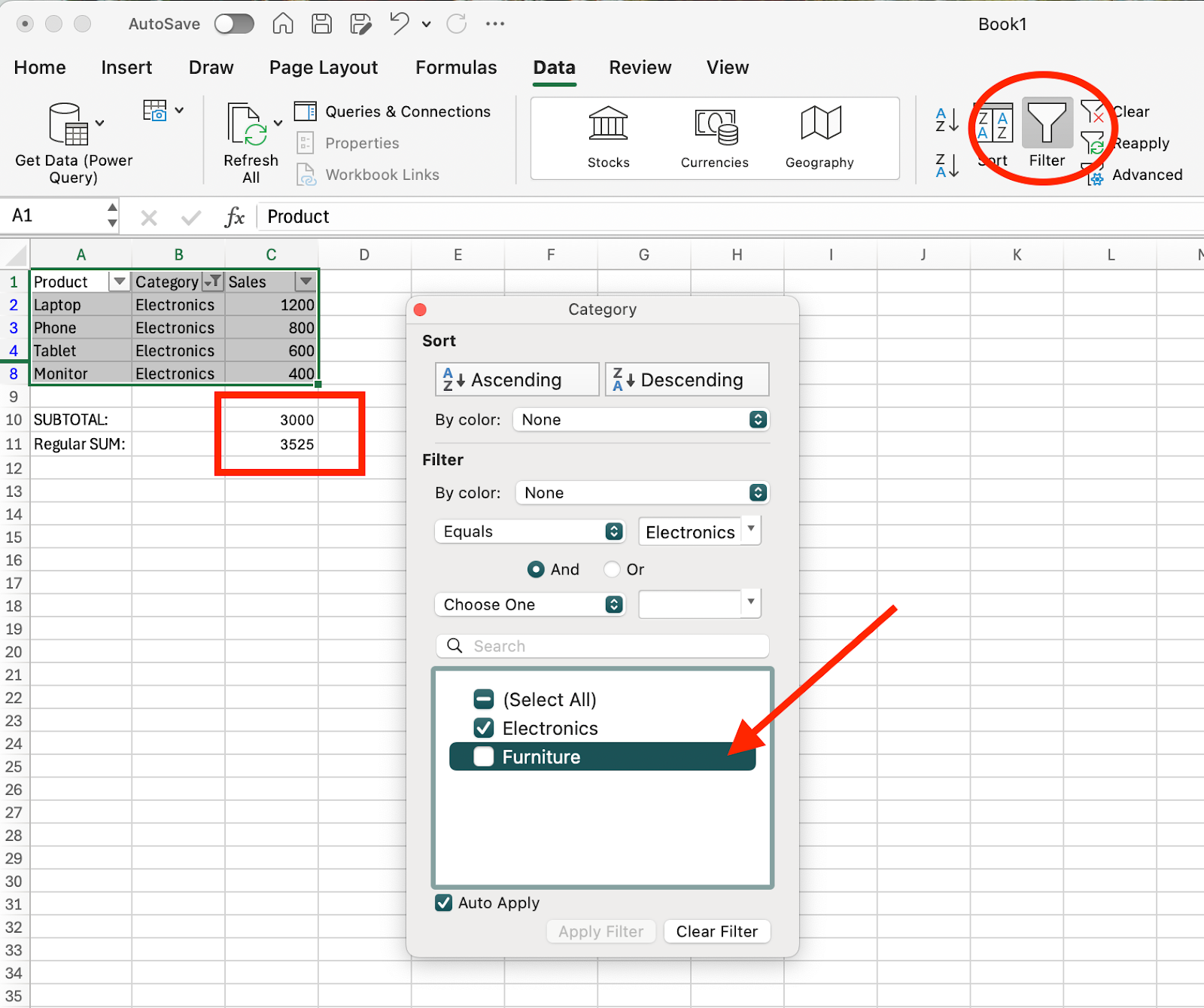Filtered Dataset. Image by Author. 

Now we've applied a filter to show only Electronics products, hiding the three Furniture rows. Notice the key difference in our calculation results:

• SUBTOTAL formula shows 3000 - automatically adjusting to sum only the visible Electronics rows
• Regular SUM formula still shows 3525 - continuing to include the hidden Furniture items

This side-by-side comparison demonstrates SUBTOTAL()'s core advantage: it responds dynamically to filters and data visibility changes, while traditional functions like SUM() remain static. When you filter data or hide rows, SUBTOTAL() recalculates instantly to reflect only what's currently visible, making it essential for responsive dashboards and interactive reports.

How SUBTOTAL() Works with Hidden and Filtered Data

The SUBTOTAL() function handles different types of hidden data in specific ways, making it essential to understand these behaviors when building your formulas.

SUBTOTAL() with filtered rows

When you apply a filter to your dataset, SUBTOTAL() always excludes the filtered-out rows from its calculations, regardless of which function number you use. This behavior is automatic and consistent across all function numbers (both 1-11 and 101-111 ranges).

For example, if you have sales data for January through December and apply a filter to show only Q1 months (January, February, March), SUBTOTAL(9, B2:B13) will calculate the sum only for those three visible months, ignoring the filtered-out Q2-Q4 data.

SUBTOTAL() with manually hidden rows

Manually hidden rows are handled differently depending on your function number choice. When you right-click on row numbers and select "Hide," you're manually hiding those rows.

Using function numbers 1-11 includes these manually hidden rows in calculations. Using function numbers 101-111 excludes them. This gives you control over whether hidden data should impact your results.

SUBTOTAL() with horizontal and vertical ranges

The SUBTOTAL() function works best with vertical data ranges (columns of data). While it can handle horizontal ranges, its hiding behavior is optimized for row-based operations since Excel's filtering and row hiding features work vertically.

When you nest SUBTOTAL() formulas within the same range, the function automatically skips other SUBTOTAL() results to avoid double counting. This is especially useful when creating hierarchical summaries or subtotals within groups, ensuring your totals accurately reflect each distinct grouping without duplication.

Advanced Uses of the SUBTOTAL() Function

Creating a dynamic dropdown summary with SUBTOTAL()

You can combine SUBTOTAL() with the IF() function to create interactive summaries that change based on user selection. This approach uses a dropdown list to let users switch between different calculation types.

To create a dynamic dropdown summary, first set up a dropdown in cell D1 with options like "Sum", "Average", "Count", and "Max".

Then, use the following formula in another cell (e.g., D2) to dynamically adjust the calculation based on the user's selection:

=IF(D1="Sum",SUBTOTAL(109,A2:A10),
  IF(D1="Average",SUBTOTAL(101,A2:A10),
  IF(D1="Count",SUBTOTAL(103,A2:A10),
  IF(D1="Max",SUBTOTAL(104,A2:A10),"Select Option"))))

This formula evaluates the dropdown selection and applies the corresponding SUBTOTAL() function. Users can switch between calculation types without editing formulas, making reports more interactive and user-friendly.

SUBTOTAL() in Excel tables and outlines

Excel Tables automatically use SUBTOTAL() in the Total Row feature. When you convert your data range to a Table (Ctrl+T) and enable the Total Row, Excel inserts SUBTOTAL(109, …) by default for sum calculations. This Total Row dynamically updates whenever rows are filtered, instantly adjusting results to reflect only visible data.

You can change the calculation type by clicking the dropdown arrow in any Total Row cell and selecting different options like Count, Average, Max, or Min. Excel automatically updates the function number while maintaining the SUBTOTAL() structure.

The Outline feature (Data > Subtotal) also relies on SUBTOTAL() formulas. When you group data and insert subtotals, Excel automatically places SUBTOTAL() functions at each group break. This creates hierarchical summaries that respond correctly when you expand or collapse outline levels, since the function ignores nested subtotal results.

Common Pitfalls and Limitations

Understanding the common errors and limitations of SUBTOTAL() helps you avoid calculation mistakes and choose the right approach for your data analysis needs.

• #VALUE! error with invalid function numbers: The most frequent error occurs when using an invalid function number. SUBTOTAL() only accepts function numbers 1-11 and 101-111. Using numbers like 12, 50, or 200 returns a #VALUE! error. Always verify your function number corresponds to a valid operation from the supported ranges.

• Hidden columns versus hidden rows behavior: While SUBTOTAL() responds to hidden rows based on your function number choice, it doesn't have the same behavior with hidden columns. The function includes data from hidden columns in all calculations, regardless of whether you use function numbers 1-11 or 101-111. This limitation means you need alternative approaches when working with datasets where column visibility affects your analysis.

• 3D references not supported: Unlike many Excel functions, SUBTOTAL() cannot reference ranges across multiple worksheets. Formulas like SUBTOTAL(109, Sheet1:Sheet3!A1:A10) return errors. As a workaround, you can first calculate sums or other aggregates separately on each sheet using standard functions like SUM(), then consolidate these intermediate results with a single SUBTOTAL on a summary sheet.

• Error values remain in calculations: SUBTOTAL() doesn't ignore cells containing error values like #N/A, #DIV/0!, or #VALUE!. These errors propagate through your subtotal calculations, potentially invalidating entire results. Clean your data of errors before applying SUBTOTAL(), or consider using the AGGREGATE() function which can skip error values.

• Vertical data orientation works best: While SUBTOTAL() can handle horizontal ranges, its design optimizes for vertical data structures. Excel's filtering, sorting, and hiding features work row-by-row, making vertical arrangements more compatible with the function's intended behavior.

Subtotal() vs. AGGREGATE()

The AGGREGATE() function serves as an enhanced alternative to SUBTOTAL() with additional capabilities for handling errors and more statistical operations. While SUBTOTAL() offers 11 basic operations, AGGREGATE() provides 19 different functions including percentiles, quartiles, and median calculations.

The primary advantage of AGGREGATE() lies in its error-handling capabilities. Unlike SUBTOTAL(), which includes error values in calculations, AGGREGATE() can automatically skip cells containing errors like #N/A, #DIV/0!, or #VALUE!. This makes it particularly useful for datasets with incomplete or problematic data.

AGGREGATE() also offers more granular control over what to ignore. You can configure it to skip hidden rows, nested subtotals, error values, or any combination of these elements using its options parameter.

Pro Tips When Using SUBTOTAL()

Always sort first

When using Excel's built-in Data > Subtotal feature, sort your data by the grouping column first. This ensures that all related records appear together, creating clean group breaks for your subtotal calculations. Unsorted data produces scattered subtotals that don't provide meaningful summaries.

Use labels in the first row of columns

Place descriptive headers in the first row of your data range before applying subtotals. Excel uses these labels to create meaningful subtotal descriptions and makes your reports easier to interpret. Clear column headers also help when selecting ranges for manual SUBTOTAL() formulas.

Be aware of summary placement (above or below)

Excel's Subtotal tool places summary rows below each group by default, but you can choose to place them above. Consider your report's intended use when making this choice. Summary rows above groups work well for executive dashboards, while summary rows below groups align with traditional accounting formats.

Hide vs. filter rows for precise control

Understand the difference between filtering and manually hiding rows to get expected results. Use filters when you want SUBTOTAL() to ignore certain data temporarily. Use manual hiding (right-click > Hide) when you want more permanent exclusions, then choose function numbers 101-111 to respect the hidden state.

This approach gives you layered control: filter for temporary data views, manually hide for semi-permanent exclusions, and select appropriate function numbers to honor your hiding intentions.

Conclusion

Learning to use SUBTOTAL() effectively transforms how you approach data analysis in Excel. Instead of creating static calculations that break when data changes, you can build resilient formulas that adapt automatically to user actions and data modifications. This skill becomes particularly valuable when working with large datasets or creating reports that multiple users will filter and manipulate over time.

To build comprehensive Excel expertise beyond individual functions like SUBTOTAL(), our Excel Fundamentals skill track provides a structured 16-hour learning path that takes you from data preparation through advanced analysis and visualization techniques. For readers ready to explore analytical applications immediately, our Data Analysis in Excel course teaches PivotTable mastery and advanced logical functions for deeper insights.