
Course
Case Study: Net Revenue Management in Excel
4 hr
5K
The SUMIFS() function in Excel adds numbers based on multiple conditions to give us precise control over calculations. Unlike SUMIF(), which checks one condition, SUMIFS() handles several conditions at once.
In this article, I’ll show you how to use SUMIFS() with advanced examples and troubleshooting tips. By the end, you’ll know how to use SUMIFS() to make your calculations more accurate and efficient.
To use the SUMIFS() function in Excel:
Type =SUMIFS( to begin the function.
Select the range that contains the values to sum.
Select the range where the condition will be applied.
Enter the condition to match.
Close the parentheses and press Enter.
Here, I have summed up all the sales that are greater than 200.
=SUMIFS(B2:B8, B2:B8, ">200")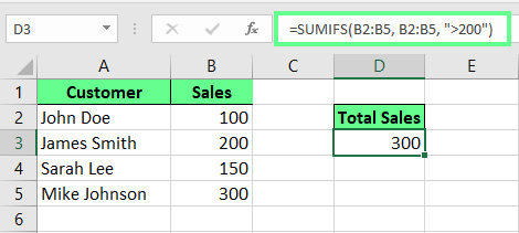
Sum up the values using the SUMIFS(). Image by Author.
The SUMIFS() function in Excel sums values only when all specified conditions are met. It supports logical operators like greater than >, less than <, equal to =, and not equal to <>, as well as wildcard characters for partial matches. The function works with numbers, text, and dates.
The SUMIFS() function first defines the range of values to sum, followed by pairs of condition ranges and criteria. Notice that SUMIFS() can handle more than one logical condition.
SUMIFS(sum_range, criteria_range1, criteria1, [criteria_range2, criteria2], …)Here:
sum_range is the range of cells you want to add.
criteria_range1 is the first range where we check for a condition.
criteria1 is the condition applied to criteria_range1.
[criteria_range2, criteria2], … are optional. You can add more pairs of ranges and conditions. Each pair adds another condition that must be met.
Note that the criteria_range (the range where conditions are checked) must have the same number of rows and columns as the sum_range (the range being summed).
Let’s try a basic example. I have a dataset of fruits with their quantities and sales. And I want to find the total sales of Apples where the Quantity is greater than 5. So my formula would become:
=SUMIFS(C2:C8, A2:A8, "Apples", B2:B8, ">5")Here C2:C8 is the range of values to sum (Sales ($)). A2:A8, "Apples" is the condition to include only rows where the product is Apples. And B2:B8, ">5" is the condition to include only rows where the Quantity exceeds 5.
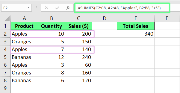
SUMIFS() formula to sum up the sales on a condition. Image by Author.
The main difference between SUMIF() and SUMIFS() is the number of conditions they use. The SUMIF() handles a single condition. But SUMIFS() can handle multiple conditions.
| Feature | SUMIF() | SUMIFS() |
|---|---|---|
| Number of conditions | Single condition only | Multiple conditions (up to 127) |
| Logic type | Simple filtering | AND logic (all conditions must be met) |
| Syntax | =SUMIF(range, criteria, [sum_range]) |
=SUMIFS(sum_range, criteria_range1, criteria1, …) |
| Argument order | Criteria range first, sum range last | Sum range first, followed by criteria pairs |
| Best used for | Simple filtering tasks | Complex data analysis with multiple criteria |
Another way to think about it is that SUMIFS() is an extension of SUMIF(). I say this because SUMIFS() can handle a single condition as well, so if you use SUMIFS() with just one condition, it functions just like SUMIF(). This means you're never technically wrong choosing SUMIFS() over SUMIF(). You can refer to our Excel formulas cheat sheet to explore more Excel formulas worth knowing.
Now that you know how the SUMIFS() function works, let's see some advanced cases where we can use this in the real world.
SUMIFS() can work with different data types like numbers, text, and dates. Let’s say I have a sales report, but some rows are missing customer names. And I want to sum up only those where we have the customer's name. For that, I use the following formula:
=SUMIFS(C2:C5, A2:A5, "<>")This formula looks at the Customer column, checks for non-blank cells, and then sums the corresponding sales.
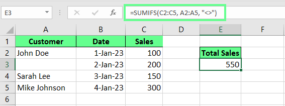
Sum up all the non-blank cells with the SUMIFS() function. Image by Author.
To sum up the sales where customer names are missing, I use this formula:
=SUMIFS(C2:C10, A2:A10, "", B2:B10, "")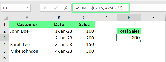
Sum up the blank cells with the SUMIFS() function. Image by Author.
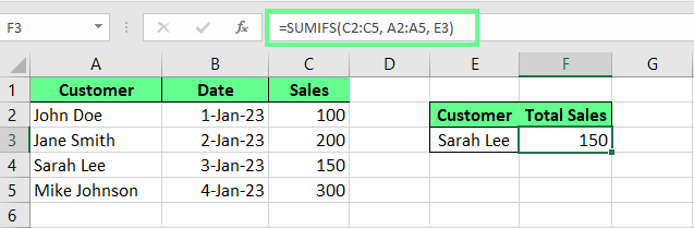
Instead of hardcoding the condition, we can store it in another cell. If I want to sum sales for Sarah Lee, I type it in cell E3 and use this formula:
=SUMIFS(C2:C5, A2:A5, E3)Whenever the value in E3 changes, the total will update automatically.
Use SUMIFS() to sum up values using the cell reference. Image by Author.
We know that SUMIFS() only uses AND logic, which means all the conditions we set must be true to add up the values. However, if we want to use OR logic, which adds up values even when any one of multiple conditions is met, we can do this by combining multiple SUMIFS().
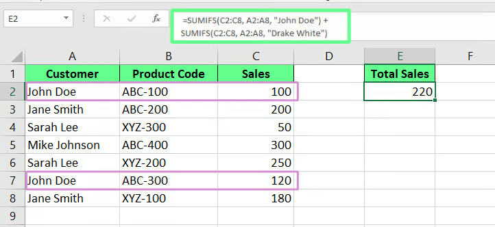
For example, if I want to sum up the sales for either John Doe OR Drake White, I combine two SUMIFS() formulas like this:
=SUMIFS(C2:C8, A2:A8, "John Doe") + SUMIFS(C2:C8, A2:A8, "Drake White")Since Drake White isn't on the list, that part of the formula returns 0. The total only includes the sales for John Doe, which shows how OR logic works.
Use OR logic in the SUMIFS() function. Image by Author.
In Excel 365 or later, we can simplify this with an array formula and it will return the same result.
=SUMIFS(C2:C8,A2:A8,{"John Doe","Drake White"})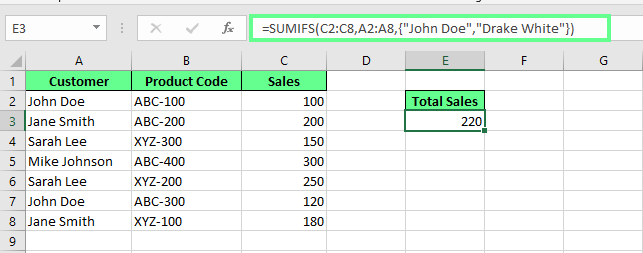
Use the SUMIFS() array formula. Image by Author.
We can also use the named ranges instead of cell references like A2:A5 or C2:C5. In this example, I select A2:A5 and name it Customer_list and select C2:C5 and name it Sales_list. Now to find the total sales of John, I use this formula:
=SUMIFS(Sales_list, Customer_list, "John")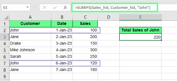
Sum up the values with the SUMIFS() using the named ranges. Image by Author.
Wildcards are special characters (* or ?) that represent unknown or variable characters in text searches and pattern matching:
* matches any number of characters (including zero).
? matches exactly one character.
Here’s how they work:
A* will match all cells that start with A.
*A will match all cells that end with A.
*A* will match all cells that contain A anywhere.
SUMIFS() function offers text-matching capabilities through wildcard characters. It identifies values that start with, end with, or contain specific text patterns. Let’s say I want to sum sales for the Product Code that starts with ABC. In this case, my formula looks like this:
=SUMIFS(D2:D8, C2:C8, "ABC*")To sum up the sales that end in 00, I write:
=SUMIFS(B2:B7, A2:A7, "*00")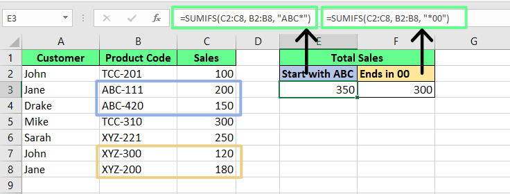
Use wildcards in SUMIFS(). Image by Author.
SUMIFS() can also sum values within a specific date range. If I want to know all sales from January 2023, I use the following formula:
=SUMIFS(D2:D8, B2:B8, ">=01-Jan-2023", B2:B8, "<=31-Jan-2023") This formula will check the dates from January 1, 2023, to January 31, 2023 and then sum up all the sales.
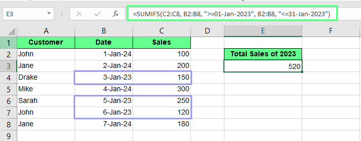
Sum up the date range using the SUMIFS(). Image by Author.
SUMIFS() function can sum values that fall within specific numerical ranges. Here, I have a random dataset and I want to sum up the values where Sales is greater than 100 but less than 300. For this, I use the following formula:
=SUMIFS(C2:C5, C2:C5, ">100", C2:C5, "<300")This formula first specifies the range of cells to sum (C2:C5) as the first argument. Then, it applies two conditions described above to the same range. The SUMIFS() function simultaneously evaluates each cell in the range against both criteria. And you can see only cells with values between 100 and 300 (exclusive) are included in the sum.
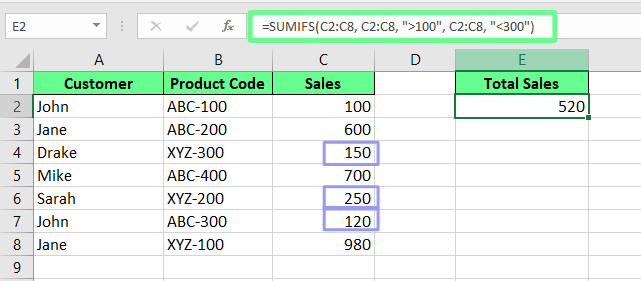
Sum up the values within a number range using the SUMIFS(). Image by Author.
If your SUMIFS() function isn’t working as expected, check for the following issues:
If your SUMIFS() formula returns an error, it may be due to mismatched range sizes. In SUMIFS(), all the ranges you select, like the sum_range and the criteria_ranges, must have the same number of rows and columns.
For example, in this formula the sum range is B2:B8, but the criteria range is A2:A7, which has one less row:
=SUMIFS(B2:B8, A2:A7, "Drake White")This mismatch will give a #VALUE! error. So, make sure all ranges are the same size, like this:
=SUMIFS(B2:B8, A2:A8, "John Doe")In SUMIFS(), you must put text criteria in quotation marks. If you don’t, it may give improper results. For example, this formula will return 0 because Excel sees Drake White as a name or variable, not as text:
=SUMIFS(B2:B8, A2:A8, Drake White)To fix it, enclose the Drake White in quotation marks like this and it will give the correct output:
=SUMIFS(B2:B8, A2:A8, "Drake White")If the formula returns 0 when you expect a result, it could be due to incorrect numerical or date-based conditions formatting. In SUMIFS(), conditions like >100 or <01-Jan-2023 must be written as text strings in quotation marks. Otherwise, it will return an error or 0 because the condition isn’t in quotes.
Or we can store the date in a separate cell (e.g., C1) and use this:
=SUMIFS(B2:B8, A2:A8, ">="&C1)SUMIFS() doesn't support certain transformations like extracting specific components from data within the formula. For example, if I want to sum up the sales of January and March, SUMIFS() won’t work directly with array criteria {"January","March"}.
To show this, suppose I have months in column A (January, February, March, April) and sales values in column B (100, 200, 300, 400). The formula
=SUMIFS(B2:B5, A2:A5, {"January","March"})won't return the expected sum of 400 (100 + 300). Instead, we can either use SUMPRODUCT():
=SUMPRODUCT((A2:A5={"January","March"})*B2:B5)or wrap SUMIFS() with SUM() using this formula:
=SUM(SUMIFS(B2:B5, A2:A5, {"January","March"}))Both solutions will correctly handle the array criteria and return the sum of sales for January and March.
To get the most out of the SUMIFS() function, we must avoid common mistakes by following these best practices:
Use wildcards for flexible filtering: It's a good practice to use wildcards when filtering the data because sometimes our data isn’t perfectly organized. Maybe product names aren’t always spelled the same way, or there are extra spaces. Wildcards help you match patterns without needing exact text.
Avoid hardcoding criteria: Instead of typing conditions directly into your formula, store them in a separate cell. If you hardcode a condition like "Drake White" or ">100", you’ll have to edit the formula every time you want to change it. However, with the cell references, the formula will update automatically.
Use absolute references when copying formulas: When you copy a SUMIFS() formula to other cells, Excel automatically adjusts the cell references. If you don’t want this to happen, use absolute references by adding $ to lock the cells in place.
SUMIFS() is an Excel function that helps us analyze data by filtering and adding up numbers that match specific criteria. It's great for tasks like tracking sales by region, summarizing expenses by category, or counting inventory by product type. Once you get comfortable with SUMIFS(), you'll realize it saves time and helps you spot important trends in your data without complicated workarounds.
If you want to build on these skills, check out our Data Analysis in Excel course, Data Preparation in Excel course, and Data Visualization in Excel course or the Excel Fundamentals skill track. They will help you brush up your existing skills.
Learn Excel with DataCamp
Course
Course
Course
Tutorial
Laiba Siddiqui
Tutorial
Vinod Chugani
Tutorial
Laiba Siddiqui
Tutorial
Laiba Siddiqui
Tutorial
Allan Ouko
Tutorial
Laiba Siddiqui