How to Sum in Excel: A Full Guide

If you use Excel, adding numbers is something you probably do a lot. It’s a key part of staying on top of budgets, tracking data, or just making sense of numbers.

We’ll show you a few different ways to sum in Excel, from quick formulas to smart Excel features, so you can use the best method that aligns with your needs.

Different Ways to Sum in Excel

There’s no one way to add data in Excel, and that’s a good thing. Depending on your work, some methods will be quicker or more helpful than others. Let’s look at five ways to sum your data.

Method 1: Using the SUM() function

The SUM() function is one of the easiest ways to add data in Excel. You can use it to total numbers, cell references, ranges, or a mix of all three.

A quick note: a cell reference is Excel’s way of pointing to a specific cell. It’s made up of the column letter and row number. For example, in the image below, the selected cell is B4, representing column B, row 4.

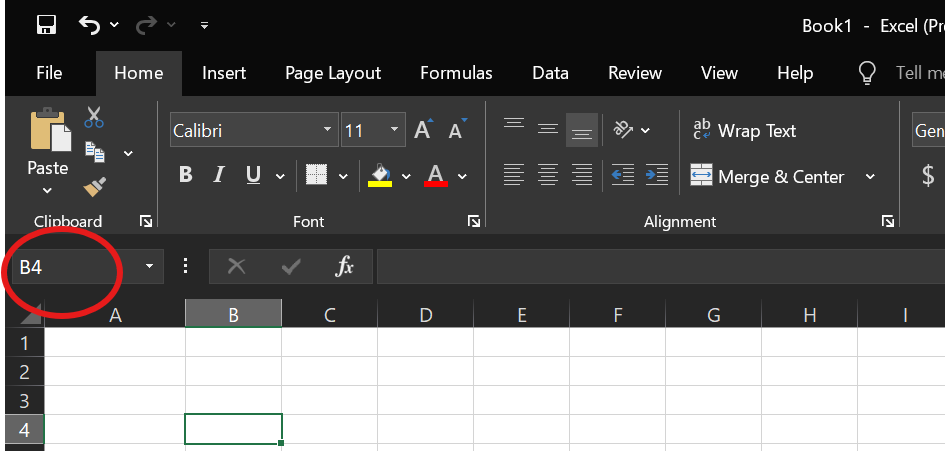
Cell reference. Image by Author

Syntax of SUM()

The SUM() function follows a basic syntax:

 = SUM(number1, [number2], ....) 

Here:

• number1 is required. It can be a number, a cell reference (like A1), or a range (like B1:B5).

• [number2] is optional and you can add as many as you like.

This function adds up all valid numbers, including both positive and negative values. Next, let’s look at a few examples to see this in action.

Sum multiple ranges

If you want to total values across two different columns, you can list both ranges in one formula:

=SUM( A1:A6, D1:D5)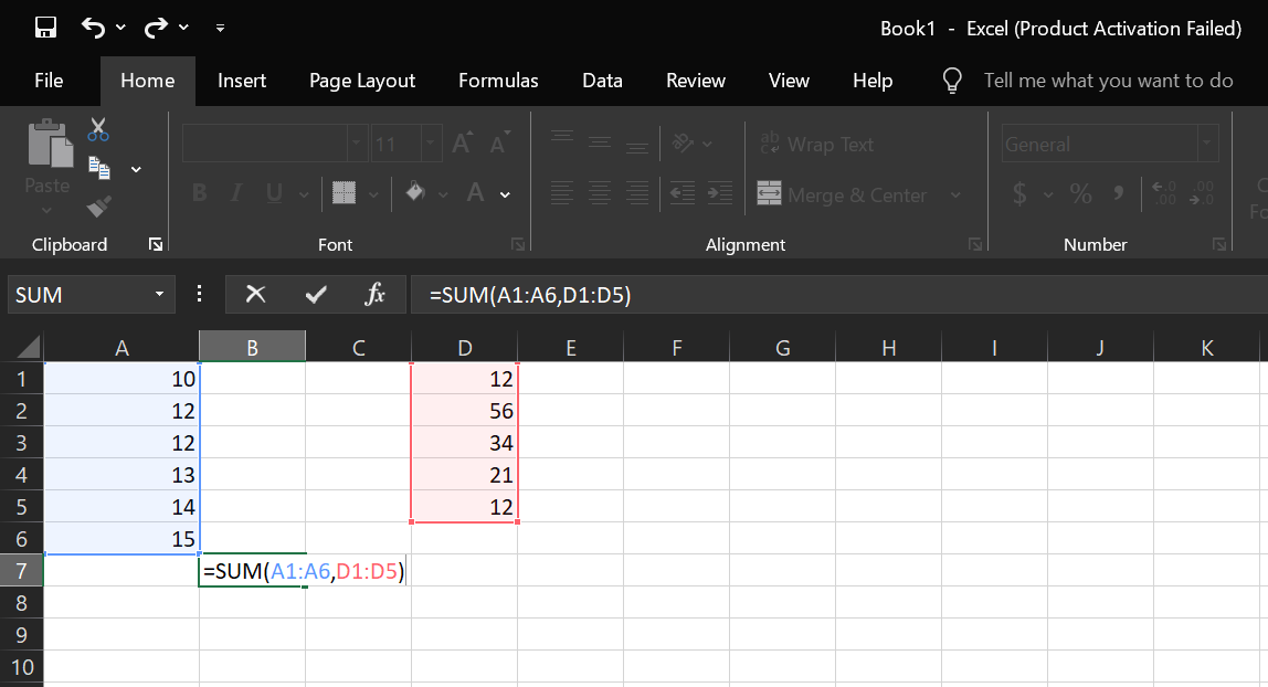 

Sum multiple ranges using SUM(). Image by Author

Sum mixed inputs

You can mix numbers, cell references, and ranges, too:

=SUM(5,A1:A5,D3)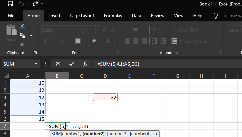 

Sum mixed inputs using SUM(). Image by Author

Method 2: Alt + = keyboard shortcut

If you want a quick way to add up your numbers without typing anything, use the Alt + = shortcut. It’s built into Excel and is one of the fastest ways to insert the SUM() function.

Here’s what it does:

• Automatically adds =SUM() below or beside your data

• Selects the range just above (for columns) or to the left (for rows)

• Works both vertically and horizontally

For example, if we're in cell A6 and the cells above (A1 to A5) contain numbers, pressing Alt + = instantly adds this formula in A6 like this:

Alt + = for inserting SUM(). Image by Author

Speed things up even more

When you work with big datasets, this shortcut can save time. And it gets even better when you combine it with another set of keys. Here’s how to sum a column fast:

1. Press Ctrl + ↓ to go to the last filled cell in a column.

2. Press ↓ once more to move to the first empty cell below.

3. Press Alt + = to insert the formula.

You can use the same trick across rows, too. And because it doesn’t involve typing, it works quickly and reduces errors.

Method 3: AutoSum feature

AutoSum is another quick way to add up numbers in Excel and like Alt + =, we don’t have to type a thing.

You’ll find the AutoSum button (∑) in two places:

• Home tab → Look for the Editing group. In the Editing Group, click the AutoSum (∑) button.

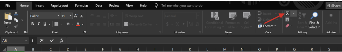
AutoSum button in the Home Tab. Image by Author

• Formulas tab → It’s the first option in the Function Library. 

AutoSum button in Formulas Tab. Image by Author

Now that we know how to access the AutoSum option, let’s see how to sum multiple columns at once using this method:

1. Select the cells where you want your totals (e.g. B7 and C7).

2. Click AutoSum.

3. Excel inserts the right formula in each:

• =SUM(B1:B6) in B7

• =SUM(C1:C6) in C7

Hit Enter, and the totals appear.

AutoSum Example. Image by Author

Method 4: Using the Status Bar for a quick sum

If you want a total fast but don’t want to write a formula, you can even use the Status Bar. When we select a column or highlight a group of cells, Excel instantly shows the sum, average, and count in the bottom-right corner of the window without typing.

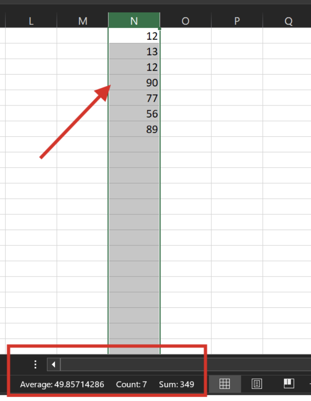
Quick Sum using Status Bar. Image by Author

By default, we see the average, count, and sum of our selected data. But you can tweak this. Right-click any of them, and the Customize Status Bar menu will pop up. From there, you can choose other values you’d like to see.

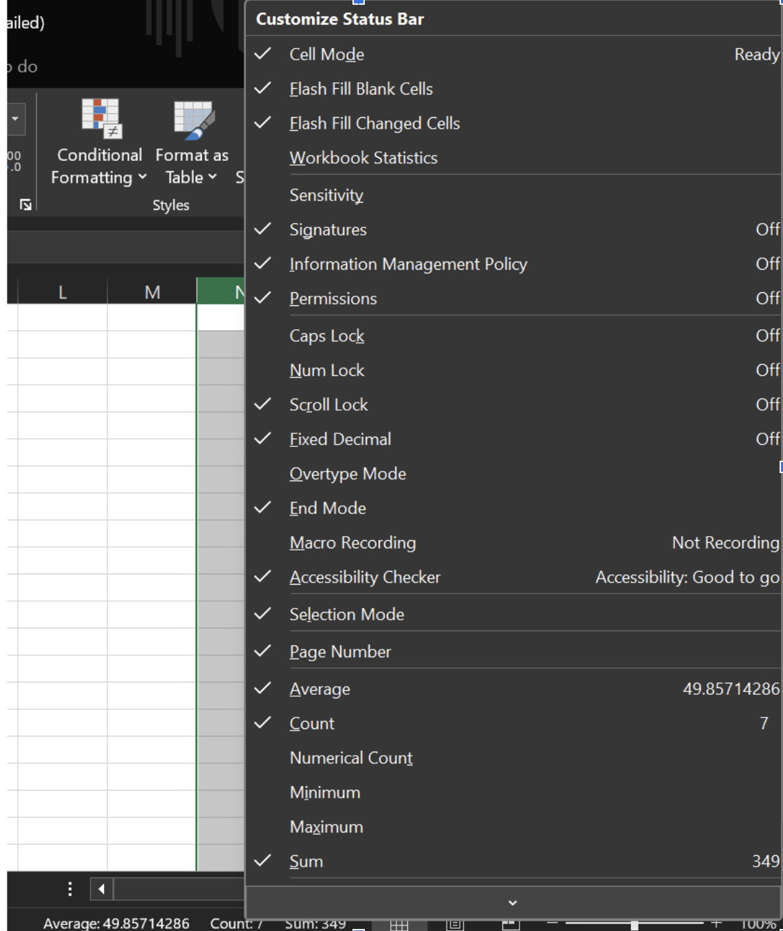
Customize Status Bar. Image by Author

However, this method helps with quick checks only and does not place the result into a cell. And if the data is filtered, the status bar will reflect only the visible (filtered) cells, not the hidden ones. This can change the sum, count, and average displayed.

Method 5: Convert data to an Excel table

We can also convert our data to an Excel table before calculating its sum. Here’s why it’s helpful:

• It updates automatically: Totals adjust as you add new rows
• It works well with filters: Only visible (filtered) data is included in totals
• You don’t need to tweak formulas: Excel handles that for you

Now, let’s see how to convert our data to an Excel table:

Step 1: Create a table using Ctrl+T

1. Select any cell within the dataset and press Ctrl + T.

2. In the Create Table dialog box, make sure the range is correct. And check the box that says My table has headers (if your data includes headers, in my case it does not).

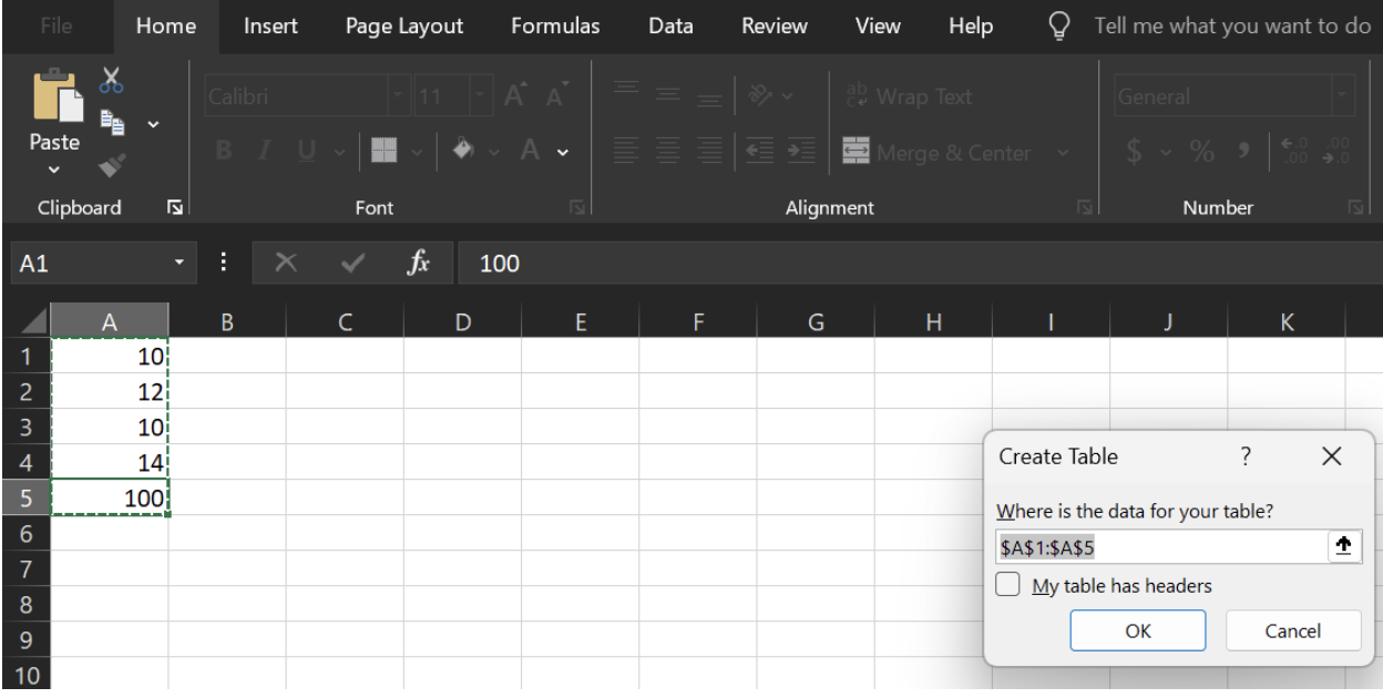
Press Ctrl+T. Image by Author.

3. Then click OK. Now your data’s in a table. You’ll see filter arrows at the top of the column.

Converting Data to Table. Image by Author.

Step 2: Enable Total Row

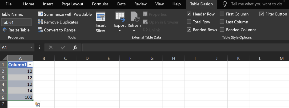
1. Click anywhere inside the table. Then, go to the Table Design tab on the ribbon. 
2. Check the Total Row box from the available options. This adds a new row at the bottom of the table.

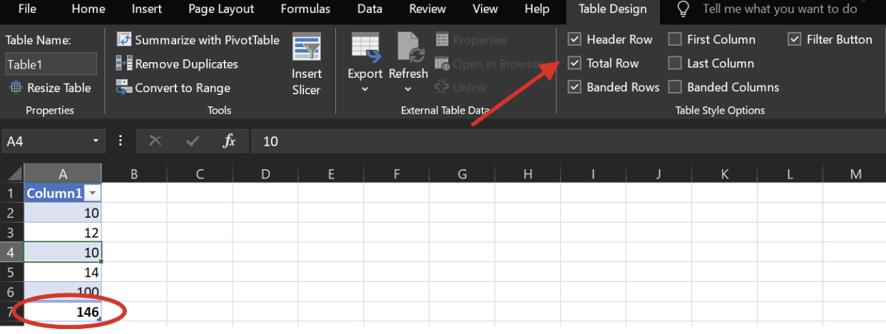
Total Row in Table Design. Image by Author

Step 3: Apply the SUM() function

1. Click the cell in the Total Row under the column you want to summarize. A drop-down menu will appear.
2. From the dropdown menu, select Sum to total that column.

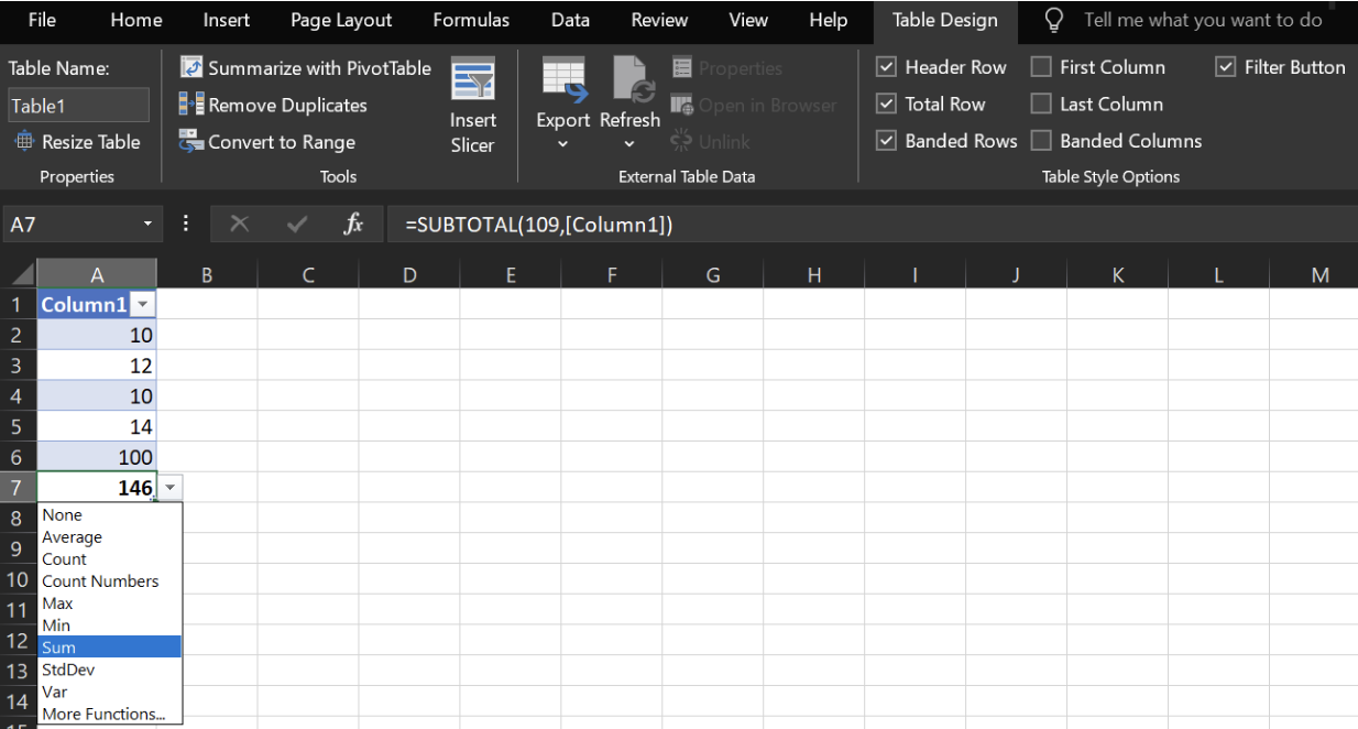
Applying the SUM() function. Image by Author

How to Sum Cells, Columns, and Rows, and by Color

Let’s now explore different cases to calculate the total of our data:

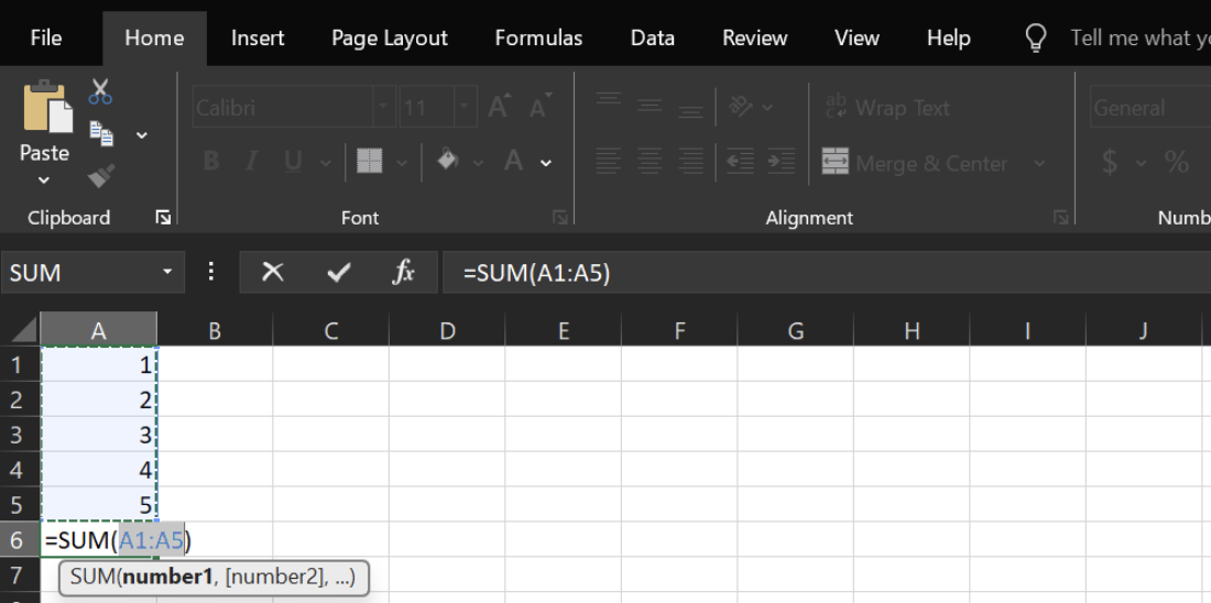
How to sum cells in Excel

Let’s say you enter some numbers in the first five cells of column A. To add them up, write:

 =SUM(A1:A5)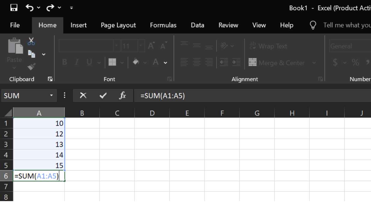

Sum a range of cells using SUM(). Image by Author

How to sum a column in Excel

To sum a column:

1. Click the empty cell right under the numbers you want to add (e.g. click B7 to sum B1 to B6)

2. Hit the AutoSum (∑) button

3. Excel highlights the range above

4. Press Enter

You’ll see =SUM(B1:B6) in the formula bar.

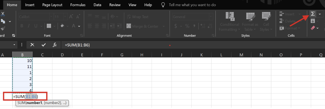
Applying AutoSum on a column. Image by Author

How to sum a row in Excel

To sum a row:

1. Click the cell to the right of the numbers (e.g. click G1 if A1 to F1 have values).

2. Click AutoSum ∑.

3. Excel selects the row automatically.

4. Press Enter.

Now you’ve got =SUM(A1:F1).

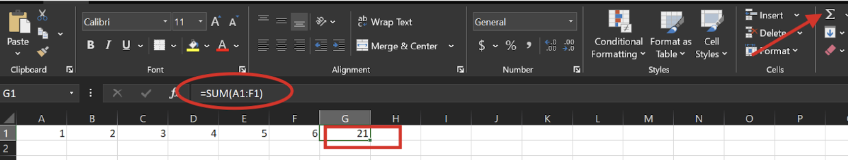
Applying AutoSum on a row. Image by Author

How to sum by color in Excel

To sum a column by color, we can pair SUMIF() with GET.Cell() function. Let’s see how:

Step 1: Create a named formula

1. Select cell C2. Go to the Formulas tab and click Name Manager.

2. In the Name Manager, click New.

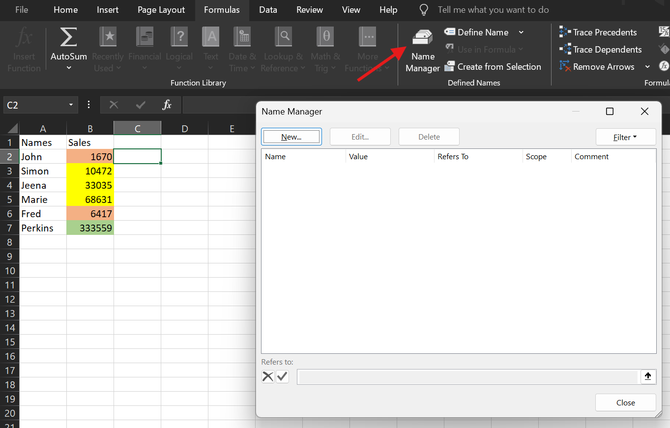
Creating a Name Manager. Image by Author

In the pop-up window:

3. Give a meaningful name like SumColor.

4. In the Refers to box, enter this formula as it tells Excel to return the fill colour index of cell B2:

= Get.Cell(38,B2)

In the function above, 38 returns a number that represents the cell's background colour from Excel’s older colour palette. It is helpful when you’re working with simple, legacy formatting.

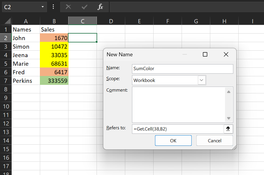
Entering details. Image by Author

Step 2: Use your named formula

Now that the name is created, we can call it in the cell.

1. Go to Cell C2 and write this formula:

= SumColor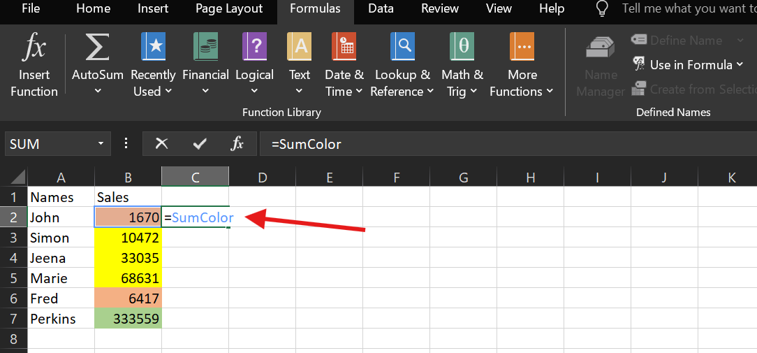

Entering the formula. Image by Author

2. Press Enter, then drag the small green square (the fill handle) down to fill the rest of the column. Now, each cell in column C shows the color code for the corresponding cell in column B.

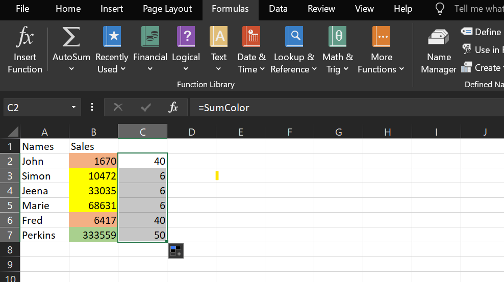
Using a Name Manager. Image by Author

Step 3: Use SUMIF() to total by color

Now, in another cell, write the SUMIF() function to add up values based on color:

=SUMIF(C2:C7, 40, B2:B7)

This example only sums values from B2:B7 where the color code in C2:C7 is 40, representing red.

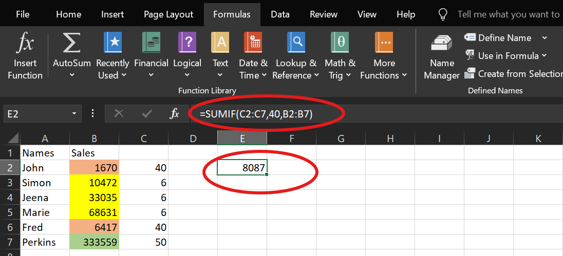
Applying SUMIF() to sum by color. Image by Author

SUM() vs. SUMIF() vs. SUMIFS()

Here’s a quick comparison of the different types of SUM() functions available in Excel:

Conclusion

As we’ve seen, there are lots of ways to sum in Excel and each one has its strengths. The SUM() function gives you more control, while Excel Tables help when we’re working with filters or growing data. AutoSum is great when you need a quick total without typing anything.

If you want to learn more, check out our Introduction to Excel course, or the Data Analysis in Excel and Data Visualization in Excel courses. The Excel Fundamentals skill track is also a great way to build confidence.