Course
Dealing With Missing Data in R
4 hr
17.2K
Multiple approaches exist for handling missing data. This section covers some of them along with their benefits and drawbacks.
To better illustrate the use case, we will be using Loan Data available on DataLab along with the source code covered in the tutorial.
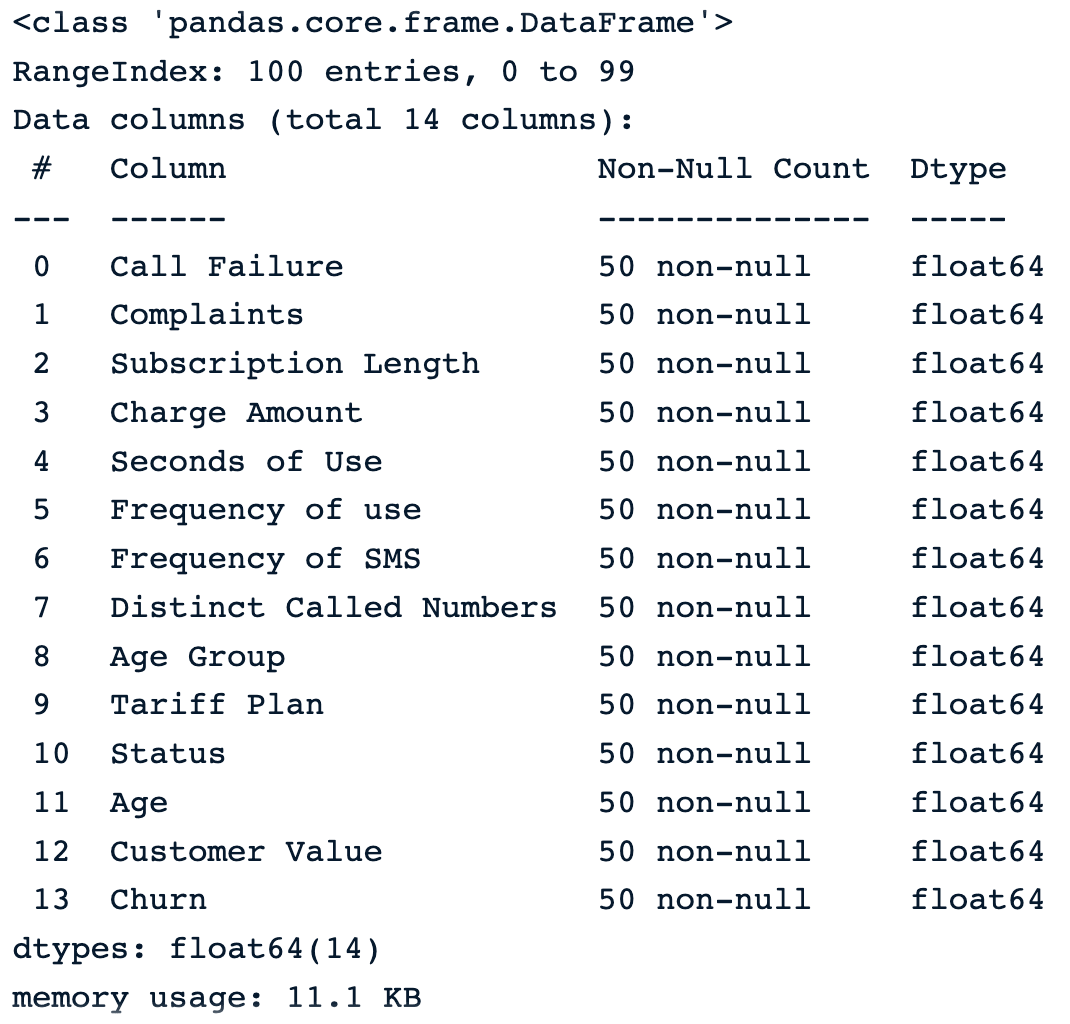
Since the dataset does not have any missing values, we will use a subset of the data (100 rows) and then manually introduce missing values.
import pandas as pdsample_customer_data = pd.read_csv("data/customer_churn.csv", nrows=100)
sample_customer_data.info()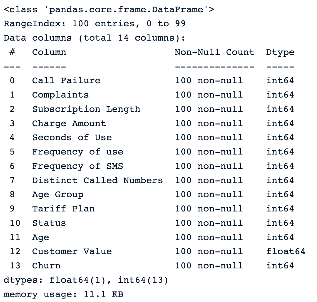
Sample of 100 random samples before introducing missing values
Let’s introduce 50% of missing values in each column of the dataframe using.
import numpy as np
def introduce_nan(x,percentage):
n = int(len(x)*(percentage - x.isna().mean()))
idxs = np.random.choice(len(x), max(n,0), replace=False, p=x.notna()/x.notna().sum())
x.iloc[idxs] = np.nan
Applying the function to the data generates this result.
sample_customer_data.apply(introduce_nan, percentage=.5)
sample_customer_data.info()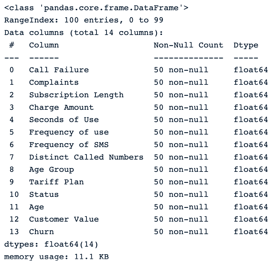
Sample of 100 random samples after introducing missing values
Below are the first five rows of the dataset.
sample_customer_data.head()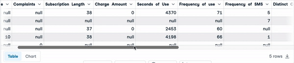
First five rows with null values
Using the dropna() function is the easiest way to remove observations or features with missing values from the dataframe. Below are some techniques.
1) Drop observations with missing values
These three scenarios can happen when trying to remove observations from a data set:
dropna(): drops all the rows with missing values.drop_na_strategy = sample_customer_data.dropna()
drop_na_strategy.info()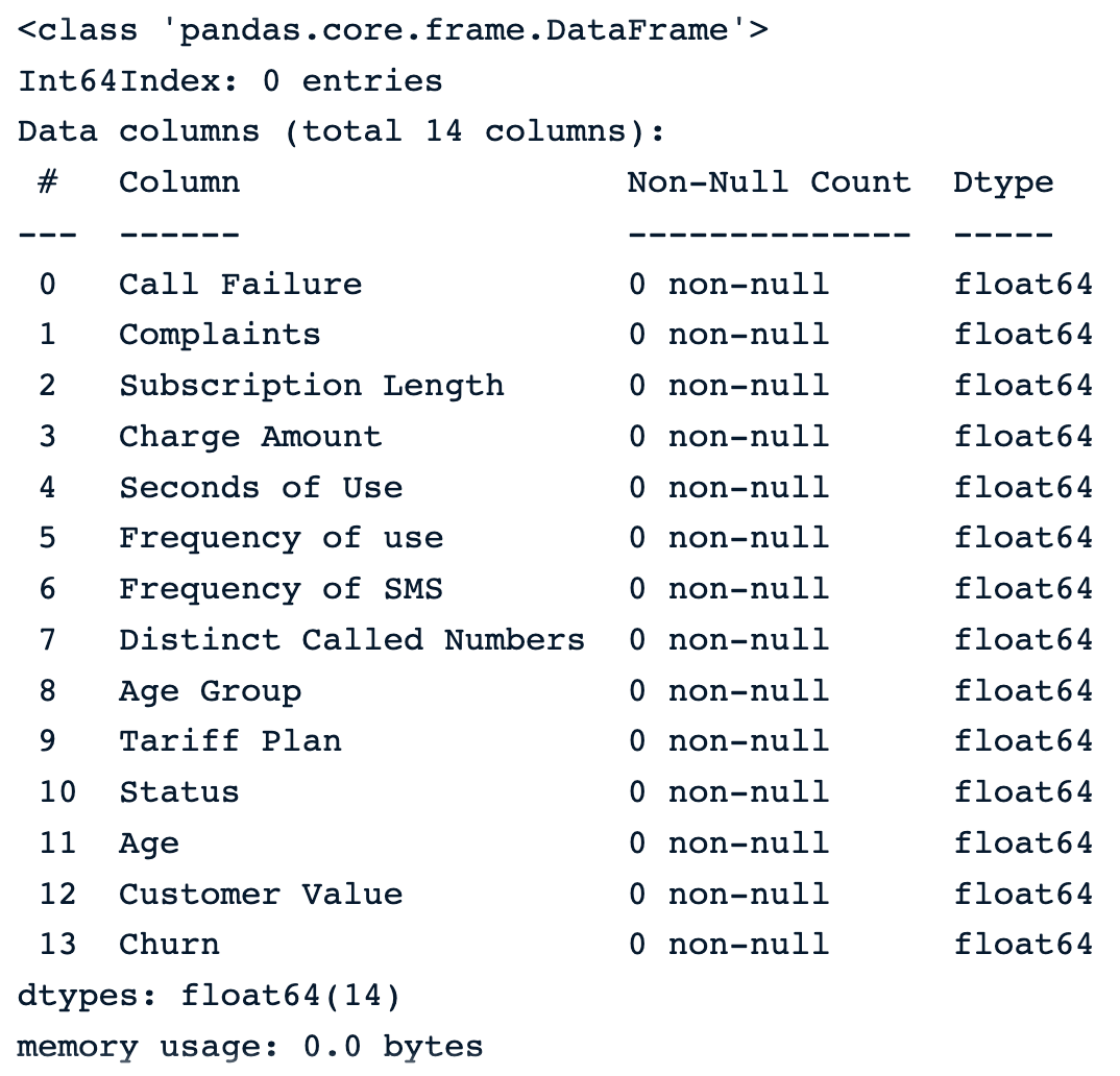
Drop observations using the default dropna() function
We can see that all the observations are dropped from the dataset, which can be especially dangerous for the rest of the analysis.
dropna(how = ‘all’): the rows where all the column values are missing.drop_na_all_strategy = sample_customer_data.dropna(how="all")
drop_na_all_strategy.info()From the output below, we notice there is no observation with all the columns missing.
Drop observations using the “all” strategy
dropna(thresh = minimum_value): drop rows based on a threshold. This strategy sets a minimum number of missing values required to preserve the rows. drop_na_thres_strategy = sample_customer_data.dropna(thresh=0.6)
drop_na_thres_strategy.info()Setting the threshold to 60%, the result is the same compared to the previous one.
Drop observations using threshold
2) Drop columns with missing values
The parameter axis = 1 can be used to explicitly specify we are interested in columns rather than rows.
dropna(axis = 1): drops all the columns with missing values.drop_na_cols_strategy = sample_customer_data.dropna(axis=1)
drop_na_cols_strategy.info()There are no more columns in the data. This is because all the columns have at least one missing value.
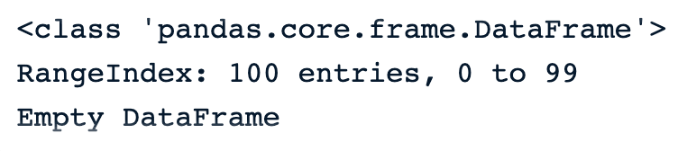
Empty dataframe after dropna() on columns
Like many other approaches, dropna() also has some pros and cons.
These replacement strategies are self-explanatory. Mean and median imputations are respectively used to replace missing values of a given column with the mean and median of the non-missing values in that column.
Normal distribution is the ideal scenario. Unfortunately, it is not always the case. This is where the median imputation can be helpful because it is not sensitive to outliers.
In Python, the fillna() function from pandas can be used to make these replacements.
mean_value = sample_customer_data.mean()
mean_imputation = sample_customer_data.fillna(mean_value)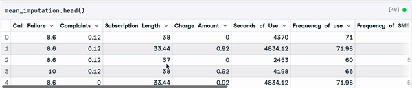
Result of the mean imputation
median_value = sample_customer_data.median()
median_imputation = sample_customer_data.fillna(median_value)
median_imputation.head()
Result of the median imputation
The idea behind the random sample imputation is different from the previous ones and involves additional steps.
def random_sample_imputation(df):

cols_with_missing_values = df.columns[df.isna().any()].tolist()

for var in cols_with_missing_values:

    # extract a random sample
    random_sample_df = df[var].dropna().sample(df[var].isnull().sum(),
                                                  random_state=0)
    # re-index the randomly extracted sample
    random_sample_df.index = df[
            df[var].isnull()].index

    # replace the NA
    df.loc[df[var].isnull(), var] = random_sample_df

return df
df = sample_customer_data.copy()
random_sample_imp_df = random_sample_imputation(sample_customer_data)
random_sample_imp_df.head()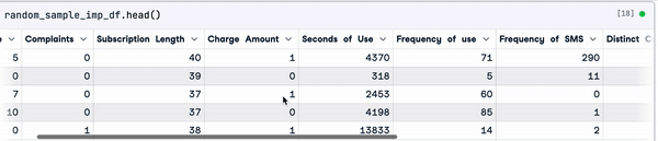
Random sample imputation
This is a multivariate imputation technique, meaning that the missing information is filled by taking into consideration the information from the other columns.
For instance, if the income value is missing for an individual, it is uncertain whether or not they have a mortgage. So, to determine the correct value, it is necessary to evaluate other characteristics such as credit score, occupation, and whether or not the individual owns a house.
Multiple Imputation by Chained Equations (MICE for short) is one of the most popular imputation methods in multivariate imputation. To better understand the MICE approach, let’s consider the set of variables X1, X2, … Xn, where some or all have missing values.
The algorithm works as follows:
The implementation is performed using the miceforest library.
First, we need to install the library using the pip.
pip install miceforestThen we import the ImputationKernel module and create the kernel for imputation.
from miceforest import ImputationKernel

mice_kernel = ImputationKernel(
data = sample_customer_data,
save_all_iterations = True,
random_state = 2023
)
Furthermore, we run the kernel on the data for two iterations, and finally, create the imputed data.
mice_kernel.mice(2)
mice_imputation = mice_kernel.complete_data()
mice_imputation.head()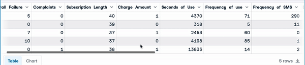
Multiple imputation
From all the imputations, it is possible to identify which one is closer to the distribution of the original data.
The mean (in yellow) and median (in red) are far away from the original distribution of the “Charge amount” column data, hence are not considered to be great for imputing the data.
mean_imputation["Charge Amount Mean Imp"] = mean_imputation["Charge Amount"]
median_imputation["Charge Amount Median Imp"] = median_imputation["Charge Amount"]
random_sample_imp_df["Charge Amount Random Imp"] = random_sample_imp_df["Charge Amount"]
With the new columns created for each type of imputation, we can now plot the distribution.
import matplotlib.pyplot as plt
plt.figure(figsize=(12,8))

sample_customer_data["Charge Amount"].plot(kind='kde',color='blue')
mean_imputation["Charge Amount Mean Imp"].plot(kind='kde',color='yellow')
median_imputation["Charge Amount Median Imp"].plot(kind='kde',color='red')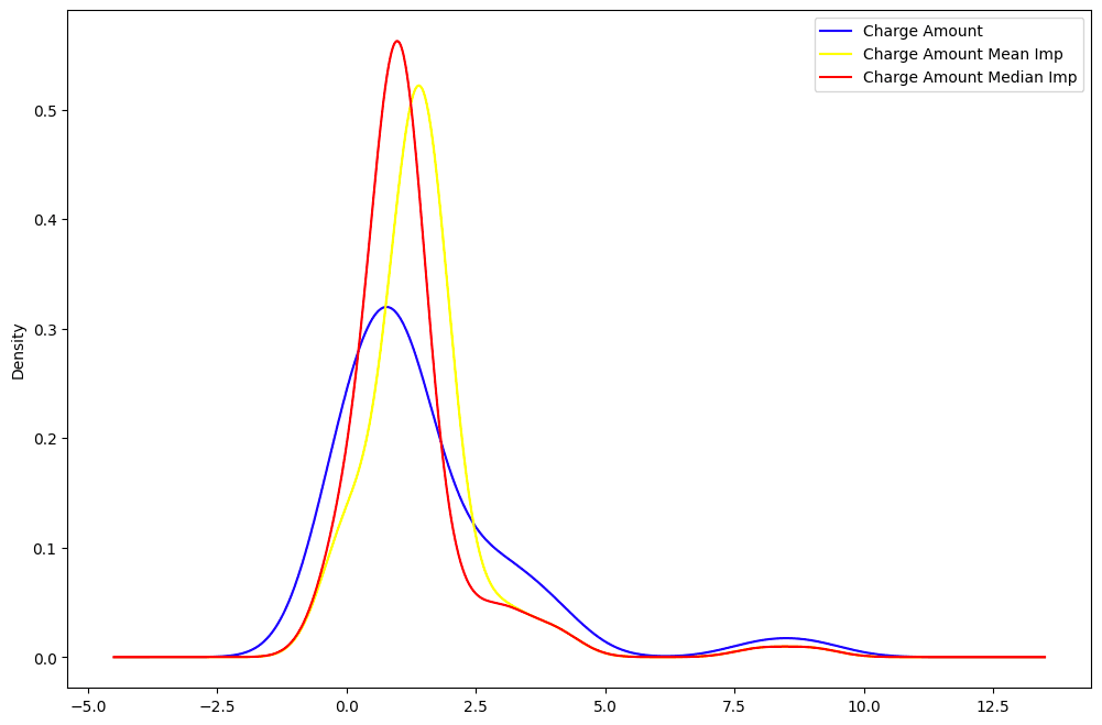
“Charge Amount” distribution: original data vs. mean vs. median.
Plotting the multiple imputation and the random imputation below, these distributions are perfectly overlapped with the original data. This means that those imputations are better than the mean and median imputations.
random_sample_imp_df["Charge Amount Random Imp"] = random_sample_imp_df["Charge Amount"]
mice_imputation["Charge Amount MICE Imp"] = mice_imputation["Charge Amount"]

mice_imputation["Charge Amount MICE Imp"].plot(kind='kde',color='black')
random_sample_imp_df["Charge Amount Random Imp"].plot(kind='kde',color='purple')

plt.legend()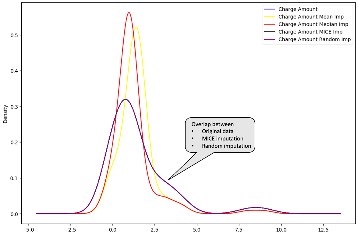
“Charge Amount” distribution: original data vs. mean vs. median vs. MICE vs.random
The Handling Missing Data with Imputations in R course is a great resource to learn more about strategies to handle missing values. It covers how to apply visualization and statistical tests to recognize missing data patterns and how to impute them with both statistical and machine learning technics.
On the same note, the dealing with missing data in python course explains how to identify, analyze, remove, and impute missing data in Python.
There are multiple imputation strategies, and they should not be used blindly. Adopting the right approach can save from introducing bias in the data and making wrong decisions.
The following table illustrates which imputation method to use based on the type of missing data. The list of methods is not exhaustive, but these are the most commonly used.
|
Type of missing data |
Imputation method |
|
Missing Completely At Random |
Mean, Median, Mode, or any other imputation method |
|
Missing At Random |
Multiple imputation, Regression imputation |
|
Missing Not At Random |
Pattern Substitution, Maximum Likelihood estimation |
It is important to keep in mind that the original data can not be recovered no matter the imputation technique. However, it is possible to use techniques that can generate imputed data sets that are as close as possible to reality.
Below are a few key steps to consider during the assessment.
Having good quality data is the goal of any stakeholders and data practitioners.
Honesty and transparency are key when communicating data missing from the analysis. Below are some important aspects to consider.
This article has covered what missing data is and its impact on the data-driven decision-making process. It has also walked you through some strategies to handle them, along with their advantages and drawbacks for actionable decision-making.
We hope it provides you with the relevant strategies to efficiently deal with your missing data issues.
Validate your professional data scientist skills.

Top Courses
Course
Course
blog
Thaylise Nakamoto
9 min
blog
Kurtis Pykes
10 min
Tutorial
Adel Nehme
Tutorial
Sayak Paul
Tutorial
Javier Canales Luna
Tutorial
Amberle McKee