Course
This tutorial is a write-up of a Facebook Live event we did a week ago. The topic was "Introduction to the Tidyverse" and this tutorial will take you through all of the content we covered during the code-along session!
You can watch the first part of the session here:
And the second part here:
Note that you can find all the code for the session in this repository.
The core tidyverse includes the packages that you're likely to use in everyday data analyses, such as ggplot2 for data visualization and dplyr for data wrangling. You'll focus on these two in this tutorial.
Remember that a package is essentially a set of tools for doing stuff with data. If you'd like to know more about packages in R, check out this tutorial.
For more on the Tidyverse, check out David Robinson's Introduction to Tidyverse course on DataCamp and the Learn the Tidyverse resources.
Getting Started
To start off, you should install the tidyverse, if you haven't already:
# Install the tidyverse
# install.packages("tidyverse")
Now that you've installed the tidyverse, it's time to load your data and check out some of the observations.
In this tutorial, you'll be exploring the Titanic dataset, where each observation is a person and each variable is a feature such as Name, Age and Survived (or not).
Load your data like this:
 # Import the Tidyverse
library(tidyverse)

# Import data
passengers <- read.csv("data/train.csv")

# Check out the first several observations of your dataframe
passengers

##   PassengerId Survived Pclass
## 1           1        0      3
## 2           2        1      1
## 3           3        1      3
## 4           4        1      1
## 5           5        0      3
## 6           6        0      3
##                                                  Name    Sex Age SibSp
## 1                             Braund, Mr. Owen Harris   male  22     1
## 2 Cumings, Mrs. John Bradley (Florence Briggs Thayer) female  38     1
## 3                              Heikkinen, Miss. Laina female  26     0
## 4        Futrelle, Mrs. Jacques Heath (Lily May Peel) female  35     1
## 5                            Allen, Mr. William Henry   male  35     0
## 6                                    Moran, Mr. James   male  NA     0
##   Parch           Ticket    Fare Cabin Embarked
## 1     0        A/5 21171  7.2500              S
## 2     0         PC 17599 71.2833   C85        C
## 3     0 STON/O2. 3101282  7.9250              S
## 4     0           113803 53.1000  C123        S
## 5     0           373450  8.0500              S
## 6     0           330877  8.4583              Q
Note that the path that you will give to read.csv() can change depending on your setup. If you'd like to just keep the same file path, you can always check out the folder structure of this project in our GitHub repository, which you can find here.
Note also that if you want to know more about all the variables that you see as a result of executing passengers, you can take a look at the dataset description.
To get an overview of your data, you can use the summary() function:
# Summarize titanic
summary(passengers)

##   PassengerId       Survived          Pclass
##  Min.   :  1.0   Min.   :0.0000   Min.   :1.000
##  1st Qu.:223.5   1st Qu.:0.0000   1st Qu.:2.000
##  Median :446.0   Median :0.0000   Median :3.000
##  Mean   :446.0   Mean   :0.3838   Mean   :2.309
##  3rd Qu.:668.5   3rd Qu.:1.0000   3rd Qu.:3.000
##  Max.   :891.0   Max.   :1.0000   Max.   :3.000
##
##                                     Name         Sex           Age
##  Abbing, Mr. Anthony                  :  1   female:314   Min.   : 0.42
##  Abbott, Mr. Rossmore Edward          :  1   male  :577   1st Qu.:20.12
##  Abbott, Mrs. Stanton (Rosa Hunt)     :  1                Median :28.00
##  Abelson, Mr. Samuel                  :  1                Mean   :29.70
##  Abelson, Mrs. Samuel (Hannah Wizosky):  1                3rd Qu.:38.00
##  Adahl, Mr. Mauritz Nils Martin       :  1                Max.   :80.00
##  (Other)                              :885                NA's   :177
##      SibSp           Parch             Ticket         Fare
##  Min.   :0.000   Min.   :0.0000   1601    :  7   Min.   :  0.00
##  1st Qu.:0.000   1st Qu.:0.0000   347082  :  7   1st Qu.:  7.91
##  Median :0.000   Median :0.0000   CA. 2343:  7   Median : 14.45
##  Mean   :0.523   Mean   :0.3816   3101295 :  6   Mean   : 32.20
##  3rd Qu.:1.000   3rd Qu.:0.0000   347088  :  6   3rd Qu.: 31.00
##  Max.   :8.000   Max.   :6.0000   CA 2144 :  6   Max.   :512.33
##                                   (Other) :852
##          Cabin     Embarked
##             :687    :  2
##  B96 B98    :  4   C:168
##  C23 C25 C27:  4   Q: 77
##  G6         :  4   S:644
##  C22 C26    :  3
##  D          :  3
##  (Other)    :186
Now do the same using a pipe %>%, one of the handiest tools in the tidyverse:
# Summarize titanic using a pipe
passengers %>%
  summary()

##   PassengerId       Survived          Pclass
##  Min.   :  1.0   Min.   :0.0000   Min.   :1.000
##  1st Qu.:223.5   1st Qu.:0.0000   1st Qu.:2.000
##  Median :446.0   Median :0.0000   Median :3.000
##  Mean   :446.0   Mean   :0.3838   Mean   :2.309
##  3rd Qu.:668.5   3rd Qu.:1.0000   3rd Qu.:3.000
##  Max.   :891.0   Max.   :1.0000   Max.   :3.000
##
##                                     Name         Sex           Age
##  Abbing, Mr. Anthony                  :  1   female:314   Min.   : 0.42
##  Abbott, Mr. Rossmore Edward          :  1   male  :577   1st Qu.:20.12
##  Abbott, Mrs. Stanton (Rosa Hunt)     :  1                Median :28.00
##  Abelson, Mr. Samuel                  :  1                Mean   :29.70
##  Abelson, Mrs. Samuel (Hannah Wizosky):  1                3rd Qu.:38.00
##  Adahl, Mr. Mauritz Nils Martin       :  1                Max.   :80.00
##  (Other)                              :885                NA's   :177
##      SibSp           Parch             Ticket         Fare
##  Min.   :0.000   Min.   :0.0000   1601    :  7   Min.   :  0.00
##  1st Qu.:0.000   1st Qu.:0.0000   347082  :  7   1st Qu.:  7.91
##  Median :0.000   Median :0.0000   CA. 2343:  7   Median : 14.45
##  Mean   :0.523   Mean   :0.3816   3101295 :  6   Mean   : 32.20
##  3rd Qu.:1.000   3rd Qu.:0.0000   347088  :  6   3rd Qu.: 31.00
##  Max.   :8.000   Max.   :6.0000   CA 2144 :  6   Max.   :512.33
##                                   (Other) :852
##          Cabin     Embarked
##             :687    :  2
##  B96 B98    :  4   C:168
##  C23 C25 C27:  4   Q: 77
##  G6         :  4   S:644
##  C22 C26    :  3
##  D          :  3
## (Other) :186Tip: if you'd like to know more about the use of the pipe operator in R, you can check out this tutorial.
Do the same after dropping observations that have missing values. Here's a hint: you can concatenate pipes!
# Summarize titanic after dropping na
passengers %>%
  drop_na() %>%
  summary()

##   PassengerId       Survived          Pclass
##  Min.   :  1.0   Min.   :0.0000   Min.   :1.000
##  1st Qu.:222.2   1st Qu.:0.0000   1st Qu.:1.000
##  Median :445.0   Median :0.0000   Median :2.000
##  Mean   :448.6   Mean   :0.4062   Mean   :2.237
##  3rd Qu.:677.8   3rd Qu.:1.0000   3rd Qu.:3.000
##  Max.   :891.0   Max.   :1.0000   Max.   :3.000
##
##                                     Name         Sex           Age
##  Abbing, Mr. Anthony                  :  1   female:261   Min.   : 0.42
##  Abbott, Mr. Rossmore Edward          :  1   male  :453   1st Qu.:20.12
##  Abbott, Mrs. Stanton (Rosa Hunt)     :  1                Median :28.00
##  Abelson, Mr. Samuel                  :  1                Mean   :29.70
##  Abelson, Mrs. Samuel (Hannah Wizosky):  1                3rd Qu.:38.00
##  Adahl, Mr. Mauritz Nils Martin       :  1                Max.   :80.00
##  (Other)                              :708
##      SibSp            Parch                 Ticket         Fare
##  Min.   :0.0000   Min.   :0.0000   347082      :  7   Min.   :  0.00
##  1st Qu.:0.0000   1st Qu.:0.0000   3101295     :  6   1st Qu.:  8.05
##  Median :0.0000   Median :0.0000   347088      :  6   Median : 15.74
##  Mean   :0.5126   Mean   :0.4314   CA 2144     :  6   Mean   : 34.69
##  3rd Qu.:1.0000   3rd Qu.:1.0000   382652      :  5   3rd Qu.: 33.38
##  Max.   :5.0000   Max.   :6.0000   S.O.C. 14879:  5   Max.   :512.33
##                                    (Other)     :679
##          Cabin     Embarked
##             :529    :  2
##  B96 B98    :  4   C:130
##  C23 C25 C27:  4   Q: 28
##  G6         :  4   S:554
##  C22 C26    :  3
##  D          :  3
##  (Other)    :167
You may have noticed stylistic consistency in the code that you've written above. That's because you're adhering to a style guide. In data science and programming/coding in general, it's important to get accustomed to using a style guide asap. As Hadley Wickham puts it in the tidyverse style guide,
Good coding style is like correct punctuation: you can manage without it, butitsuremakesthingseasiertoread.
In the next section, you'll tackle data wrangling with dplyr to filter your data, arrange it and create new features by mutating old ones.
Wrangle your Data
Now it's time to explore your data and get some initial insight into the dataset. You'll be using dplyr verbs such as filter(), arrange() and mutate(), which do exactly what they say.
Let's sat that you wanted to choose a particular set of observations, say, those for which the "Sex" was 'female'. dplyr allows us to do intuitively and in a language that mirrors how you think and talk about data.
The filter verb chooses only the observations that match the condition. See it in action:
# Filter to get all "male" rows
passengers %>%
  filter(Sex == "male")

##   PassengerId Survived Pclass                           Name  Sex Age
## 1           1        0      3        Braund, Mr. Owen Harris male  22
## 2           5        0      3       Allen, Mr. William Henry male  35
## 3           6        0      3               Moran, Mr. James male  NA
## 4           7        0      1        McCarthy, Mr. Timothy J male  54
## 5           8        0      3 Palsson, Master. Gosta Leonard male   2
## 6          13        0      3 Saundercock, Mr. William Henry male  20
##   SibSp Parch    Ticket    Fare Cabin Embarked
## 1     1     0 A/5 21171  7.2500              S
## 2     0     0    373450  8.0500              S
## 3     0     0    330877  8.4583              Q
## 4     0     0     17463 51.8625   E46        S
## 5     3     1    349909 21.0750              S
## 6     0     0 A/5. 2151  8.0500              S
When looking at the results of the code chunk above, you'll see that it looks like many men didn't survive the sinking of the RMS Titanic. This is interesting, and you'll explore this more rigorously later on in this tutorial!
Note that you can read dplyr code like a sentence: take your data and then (%>%) filter it according the condition that the sex is male. The code that you see in the above code chunk does not alter the original data frame. filter(Sex = "male") is a common error (Hugo made this same mistake!); there's a cool tidyverse error guide.
# Filter to get all "female" rows
passengers %>%
  filter(Sex == "female")

##   PassengerId Survived Pclass
## 1           2        1      1
## 2           3        1      3
## 3           4        1      1
## 4           9        1      3
## 5          10        1      2
## 6          11        1      3
##                                                  Name    Sex Age SibSp
## 1 Cumings, Mrs. John Bradley (Florence Briggs Thayer) female  38     1
## 2                              Heikkinen, Miss. Laina female  26     0
## 3        Futrelle, Mrs. Jacques Heath (Lily May Peel) female  35     1
## 4   Johnson, Mrs. Oscar W (Elisabeth Vilhelmina Berg) female  27     0
## 5                 Nasser, Mrs. Nicholas (Adele Achem) female  14     1
## 6                     Sandstrom, Miss. Marguerite Rut female   4     1
##   Parch           Ticket    Fare Cabin Embarked
## 1     0         PC 17599 71.2833   C85        C
## 2     0 STON/O2. 3101282  7.9250              S
## 3     0           113803 53.1000  C123        S
## 4     2           347742 11.1333              S
## 5     0           237736 30.0708              C
## 6     1          PP 9549 16.7000    G6        S
Women seem to be more likely to have survived the Titanic disaster, at least, anecdotally speaking.
When you explore data, you should be asking and answering questions that you might be interested in to the best of your abilities! Right now, You might want to arrange() your observations by increasing Fare to see if you can notice any trends. You can use the verb arrange() to achieve this:
# Arrange by increasing Fare
passengers %>%
  arrange(Fare)

##   PassengerId Survived Pclass                            Name  Sex Age
## 1         180        0      3             Leonard, Mr. Lionel male  36
## 2         264        0      1           Harrison, Mr. William male  40
## 3         272        1      3    Tornquist, Mr. William Henry male  25
## 4         278        0      2     Parkes, Mr. Francis "Frank" male  NA
## 5         303        0      3 Johnson, Mr. William Cahoone Jr male  19
## 6         414        0      2  Cunningham, Mr. Alfred Fleming male  NA
##   SibSp Parch Ticket Fare Cabin Embarked
## 1     0     0   LINE    0              S
## 2     0     0 112059    0   B94        S
## 3     0     0   LINE    0              S
## 4     0     0 239853    0              S
## 5     0     0   LINE    0              S
## 6     0     0 239853    0              S
A lot of the people who paid less, did not survive the disaster. That's something interesting that you've just discovered just by re-arranging your data!
You can also arrange by decreasing Fare:
# Arrange by decreasing Fare
passengers %>%
  arrange(desc(Fare))

##   PassengerId Survived Pclass                               Name    Sex
## 1         259        1      1                   Ward, Miss. Anna female
## 2         680        1      1 Cardeza, Mr. Thomas Drake Martinez   male
## 3         738        1      1             Lesurer, Mr. Gustave J   male
## 4          28        0      1     Fortune, Mr. Charles Alexander   male
## 5          89        1      1         Fortune, Miss. Mabel Helen female
## 6         342        1      1     Fortune, Miss. Alice Elizabeth female
##   Age SibSp Parch   Ticket     Fare       Cabin Embarked
## 1  35     0     0 PC 17755 512.3292                    C
## 2  36     0     1 PC 17755 512.3292 B51 B53 B55        C
## 3  35     0     0 PC 17755 512.3292        B101        C
## 4  19     3     2    19950 263.0000 C23 C25 C27        S
## 5  23     3     2    19950 263.0000 C23 C25 C27        S
## 6  24     3     2    19950 263.0000 C23 C25 C27        S
There are indeed more survivors at the top end!
Sometimes you may wish to create new variables. You know that the variable Parch is the number of parents and children while SibSp is the number of siblings and spouses. You can add these together to get a new variable FamSize. This is feature engineering and it's a big part of machine learning a lot of the time!
Now, to make your new variable, you mutate() the original variables into the new one.
# Create new column FamSize (size of family)
passengers %>%
  mutate(FamSize = Parch + SibSp)

##   PassengerId Survived Pclass
## 1           1        0      3
## 2           2        1      1
## 3           3        1      3
## 4           4        1      1
## 5           5        0      3
## 6           6        0      3
##                                                  Name    Sex Age SibSp
## 1                             Braund, Mr. Owen Harris   male  22     1
## 2 Cumings, Mrs. John Bradley (Florence Briggs Thayer) female  38     1
## 3                              Heikkinen, Miss. Laina female  26     0
## 4        Futrelle, Mrs. Jacques Heath (Lily May Peel) female  35     1
## 5                            Allen, Mr. William Henry   male  35     0
## 6                                    Moran, Mr. James   male  NA     0
##   Parch           Ticket    Fare Cabin Embarked FamSize
## 1     0        A/5 21171  7.2500              S       1
## 2     0         PC 17599 71.2833   C85        C       1
## 3     0 STON/O2. 3101282  7.9250              S       0
## 4     0           113803 53.1000  C123        S       1
## 5     0           373450  8.0500              S       0
## 6     0           330877  8.4583              Q       0
Note that mutate() can be used to create new columns but also modify existing columns in much the same way that a mutation may from a biological perspective. It's not exactly right but a nice way to provide context for verb choice.
Now that you have your extra variable, you can ask other questions, such as "Is it possible that larger family have a lower rate of survival?".
To test this hypothesis, create a new variable FamSize as the sum of Parch and SibSp as above, then arrange by decreasing FamSize:
# Create new column FamSize (size of family)
# Arrange by decreasing FamSize
passengers %>%
  mutate(FamSize = Parch + SibSp) %>%
  arrange(desc(FamSize))

##   PassengerId Survived Pclass                         Name    Sex Age
## 1         160        0      3   Sage, Master. Thomas Henry   male  NA
## 2         181        0      3 Sage, Miss. Constance Gladys female  NA
## 3         202        0      3          Sage, Mr. Frederick   male  NA
## 4         325        0      3     Sage, Mr. George John Jr   male  NA
## 5         793        0      3      Sage, Miss. Stella Anna female  NA
## 6         847        0      3     Sage, Mr. Douglas Bullen   male  NA
##   SibSp Parch   Ticket  Fare Cabin Embarked FamSize
## 1     8     2 CA. 2343 69.55              S      10
## 2     8     2 CA. 2343 69.55              S      10
## 3     8     2 CA. 2343 69.55              S      10
## 4     8     2 CA. 2343 69.55              S      10
## 5     8     2 CA. 2343 69.55              S      10
## 6     8     2 CA. 2343 69.55              S      10
Everyone in the top family did not survive! This might be telling: maybe if you're part of a large family, you weren't able to get off of the Titanic in time.
However, as zeroes and ones don't often say a great deal, mutate the values of the Survived variable to strings No and Yes (and create new data frame!):
# Turn numerical values of Survived column to "No" & "Yes" (new data frame)
passengers1 <- passengers %>%
  mutate(Survived = ifelse(Survived == 0, "No", "Yes"))
passengers1

##   PassengerId Survived Pclass
## 1           1       No      3
## 2           2      Yes      1
## 3           3      Yes      3
## 4           4      Yes      1
## 5           5       No      3
## 6           6       No      3
##                                                  Name    Sex Age SibSp
## 1                             Braund, Mr. Owen Harris   male  22     1
## 2 Cumings, Mrs. John Bradley (Florence Briggs Thayer) female  38     1
## 3                              Heikkinen, Miss. Laina female  26     0
## 4        Futrelle, Mrs. Jacques Heath (Lily May Peel) female  35     1
## 5                            Allen, Mr. William Henry   male  35     0
## 6                                    Moran, Mr. James   male  NA     0
##   Parch           Ticket    Fare Cabin Embarked
## 1     0        A/5 21171  7.2500              S
## 2     0         PC 17599 71.2833   C85        C
## 3     0 STON/O2. 3101282  7.9250              S
## 4     0           113803 53.1000  C123        S
## 5     0           373450  8.0500              S
## 6     0           330877  8.4583              Q
Plotting your Data
To plot your data using ggplot2, you specify three things:
- Your data
- Your aesthetics (for example, what's on the x-axis)
- Your layers (for example, barplot, scatterplot)
First you'll plot a barplot of Sex to see how many males and females were recorded aboard the Titanic:
# Plot barplot of passenger Sex
ggplot(passengers, aes(x = Sex)) +
  geom_bar()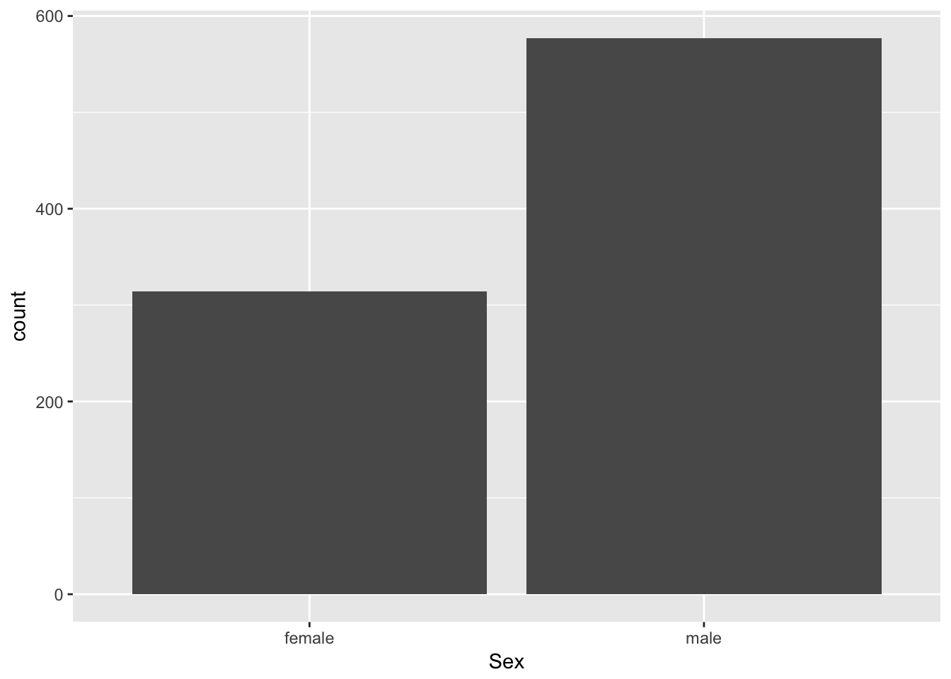
From the above plot, you can tell that there were about 600 men and 300 women aboard of the RMS Titanic.
Note that the aes() function is really a way to map the aesthetics of the plot to the variables in the data. See Modern Dive by Chester Ismay & Albert Y. Kim for more.
Now it's time for some scatter plots. Is the Age of any given passenger correlated with the Fare that they paid?
# Scatter plot of Age vs Fare
ggplot(passengers, aes(x = Age, y = Fare)) +
  geom_point()

## Warning: Removed 177 rows containing missing values (geom_point).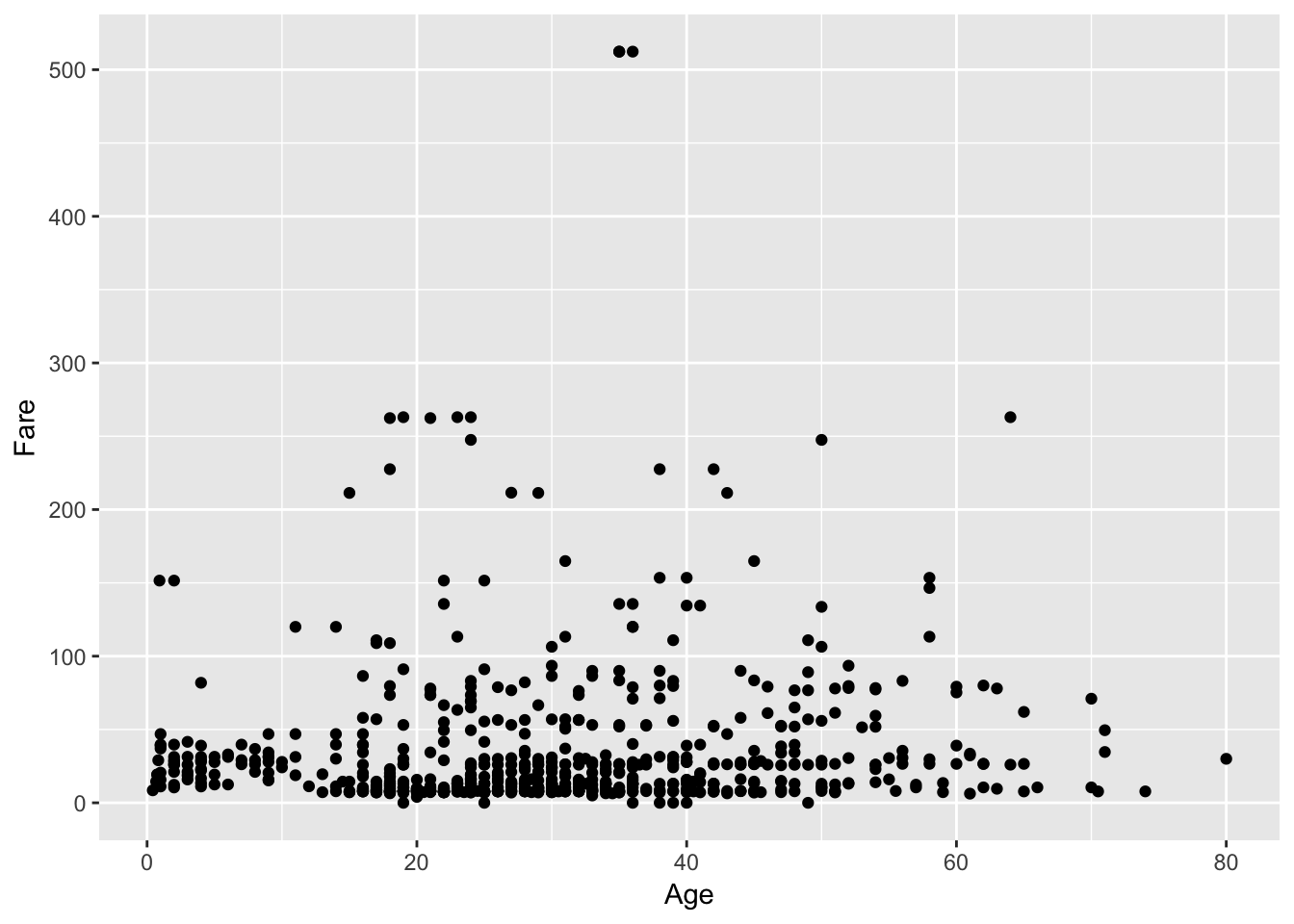
You gathered a lot of insights just from this one plot! You see that a lot of the people who paid more, were also substantially older. There might have been an increase in fare according to age... Additionally, you immediately see the two outliers on top of the plot, which you might want to investigate further!
You can read your ggplot2 code like a sentence, just like your dplyr code above: "You take the data as titanic and you map Age to the x axis and Fare to the y axis, adding points on as the layer of the plot."
Let's take the previous plot and color each point by Sex, to see any correlations between Sex, Age and Fare:
# Scatter plot of Age vs Fare colored by Sex
ggplot(passengers %>% drop_na(), aes(x = Age, y = Fare, color = Sex)) +
  geom_point()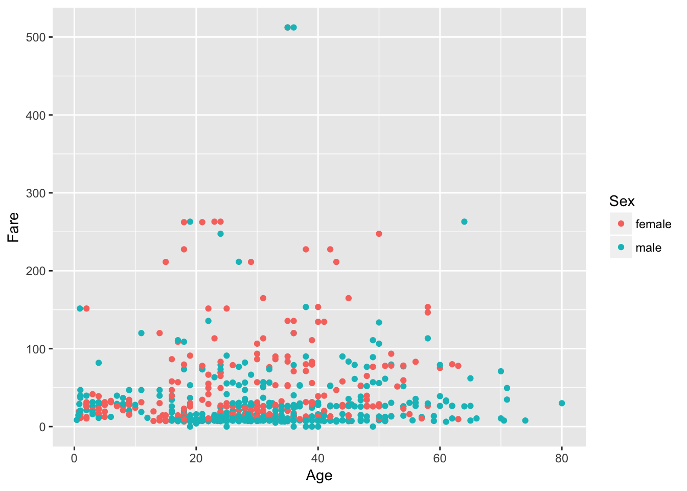
You see that a lot of the people down the bottom, who paid less, were men. You also have a cluster of women towards the top of the plot that were slightly older and also paid more to get on board of the Titanic.
Visualizing three variables (two numeric ones, Age and Fare, and one categorical one, Sex) on one plot is pretty cool, but what if you wanted to throw the Survived variable into the mix to see if there are any apparent trends? You can do this with faceting, which is a way to produce multiple plots simultaneously:
# Scatter plot of Age vs Fare colored by Sex faceted by Survived
ggplot(passengers1, aes(x = Age, y = Fare, color = Sex)) +
  geom_point() +
  facet_grid(~Survived)

## Warning: Removed 177 rows containing missing values (geom_point).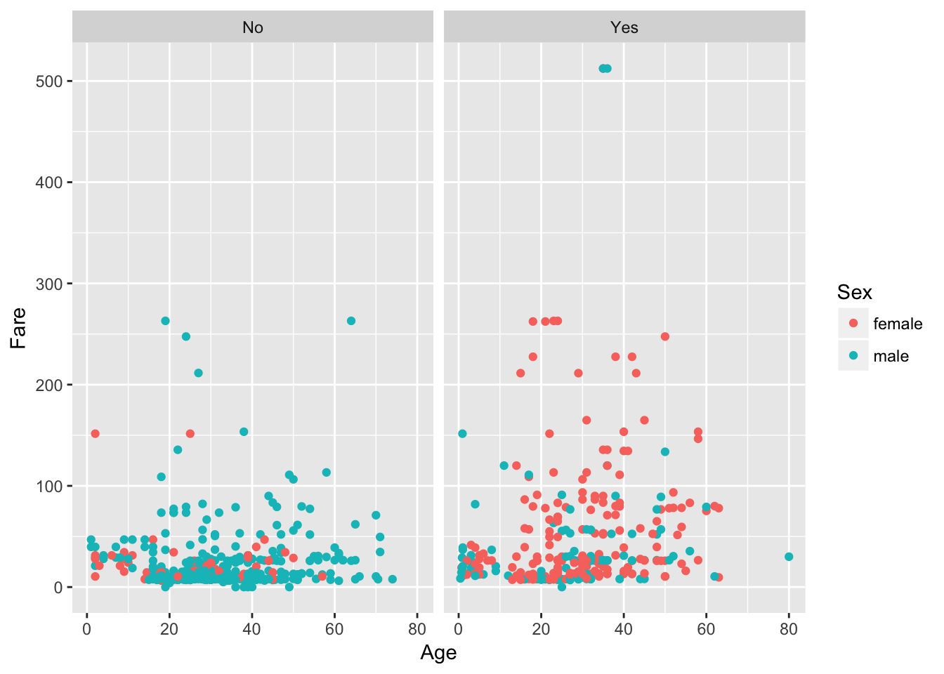
Suddenly, you see that a lot of the women who you noted up there in the previous plot have survived, and that most of them who didn't survive, paid under 50 units. Tip: try to figure out the units of the currency yourself!
Now let's redo your bar plot of passenger Sex and this time fill your bars according to Survived:
# Plot barplot of passenger Sex & fill according to Survival
ggplot(passengers1, aes(x = Sex, fill = Survived)) +
  geom_bar()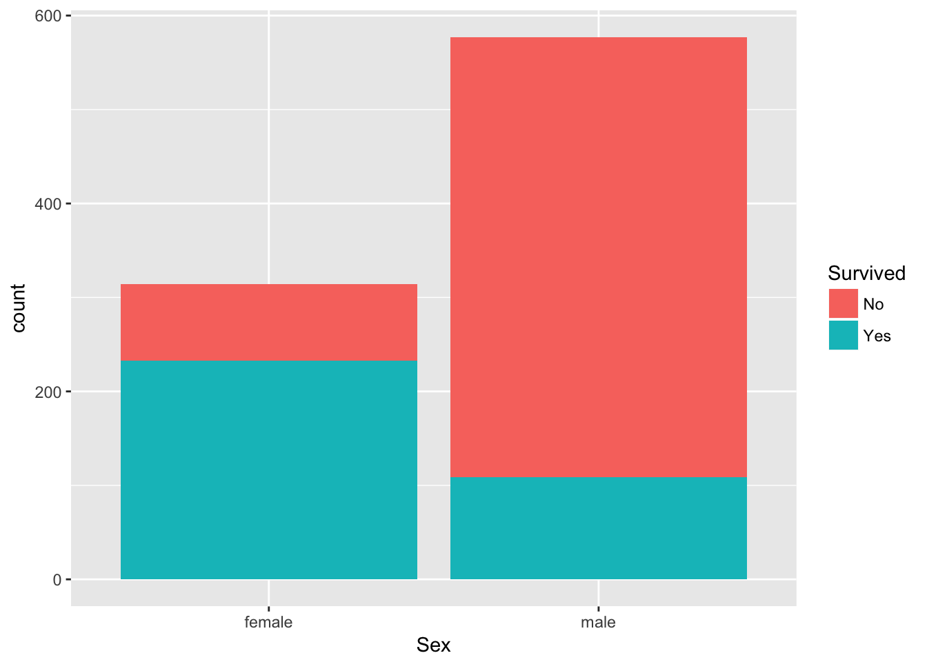
You see that the vast proportion of men did not survive, whereas over two-thirds of the women did survive!
Summarizing and Grouping your Data
Use the summarise() verb to find out the mean fare paid:
# Check out mean Fare
passengers %>%
  summarise(meanFare = mean(Fare))

##   meanFare
## 1 32.20421
Use the summarise() verb to find out the median fare paid:
# Check out mean Fare
passengers %>%
  summarise(medianFare = median(Fare))

##   medianFare
## 1    14.4542
You can also use the filter() and summarise() verbs to find out the mean fare paid among men:
# Check out mean Fare for men
passengers %>%
  filter(Sex == "male") %>%
  summarise(meanFare = mean(Fare))

##   meanFare
## 1 25.52389
Use the filter() and summarise() verbs to find out the mean fare paid among women:
# Check out mean Fare for women
passengers %>%
  filter(Sex == "female") %>%
  summarise(meanFare = mean(Fare))

##   meanFare
## 1 44.47982
Use the filter() and summarise() verbs to find out the mean fare paid among women and how many women survived:
# Check out mean Fare & number of survivors for women
passengers %>%
  filter(Sex == "female") %>%
  summarise(meanFare = mean(Fare), numSurv = sum(Survived))

##   meanFare numSurv
## 1 44.47982     233
Use the group_by() and summarise() verbs to find the mean fare and number of survivors as a function of sex:
# Check out mean Fare & number of survivors grouped by Sex
passengers %>%
  group_by(Sex) %>%
  summarise(meanFare = mean(Fare), numSurv = sum(Survived))

## # A tibble: 2 x 3
##   Sex    meanFare numSurv
##   <fct>     <dbl>   <int>
## 1 female     44.5     233
## 2 male       25.5     109
Use the group_by() and summarise() verbs to find the mean fare and proportion of survivors as a function of sex:
# Check out mean Fare & proportion of survivors grouped by Sex
passengers %>%
  group_by(Sex) %>%
  summarise(meanFare = mean(Fare), numSurv = sum(Survived)/n())

## # A tibble: 2 x 3
##   Sex    meanFare numSurv
##   <fct>     <dbl>   <dbl>
## 1 female     44.5   0.742
## 2 male       25.5   0.189
Conclusion
In this tutorial, you have gone from zero to one with the basics of data analysis using the tidyverse and tidy tools. You've learnt how to filter() your data, arrange() and mutate() it, plot and summarise() it using dplyr and ggplot2, all by writing code that mirrors the way you think and talk about data. Congratulations. I'd encourage you to learn more by taking David Robinson's Introduction to Tidyverse course and by using these tools on other datasets that interest you. Share these analyses with us on twitter @DataCamp and @hugobowne. Thanks for reading.
