Machine Learning Basics - The Norms

Introduction

Linear algebra is one of the basic mathematical tools that we need in data science. Having some comprehension of these concepts can increase your understanding of various algorithms. It really is an excellent basis for a data science/machine learning path.

The goal of this tutorial is to enter mathematics for data science by coding with Python/Numpy. I think that having practical tutorials on theoretical topics like linear algebra can be useful because writing and reading code is a good way to truly understand mathematical concepts. And above all, I think that it can be a lot of fun!

There are no particular prerequisites, but if you are not sure what a matrix is or how to do the dot product, the first posts (1 to 4) of my series on the deep learning book by Ian Goodfellow are a good start.

In this tutorial, we will approach an important concept for machine learning and deep learning: the norm. The norm is extensively used, for instance, to evaluate the goodness of a model. By the end of this tutorial, you will hopefully have a better intuition of this concept and why it is so valuable in machine learning. We will also see how the derivative of the norm is used to train a machine learning algorithm.

Basic Setup

Before all, we will setup the libraries that we will use:

import numpy as np
import matplotlib.pyplot as plt
import seaborn as sns

And add some Latex shortcut to the commands bs for bold symbols and norm for the symbol of the norm:

$$
\newcommand\bs[1]{\boldsymbol{#1}}
\newcommand\norm[1]{\left\lVert#1\right\rVert}
$$

$$ \newcommand\bs[1]{\boldsymbol{#1}} \newcommand\norm[1]{\left\lVert#1\right\rVert} $$

The last thing to setup is the appearance of the graphics that we will create:

# Plot parameters
sns.set()
%pylab inline
pylab.rcParams['figure.figsize'] = (4, 4)
plt.rcParams['xtick.major.size'] = 0
plt.rcParams['ytick.major.size'] = 0

Populating the interactive namespace from numpy and matplotlib

A Practical Example

Let's start with a simple example. Imagine that you have a dataset of songs containing different features. Now let's say that you want to build a model that predicts the duration of a song according to other features like the genre of music, the instrumentation, etc. You trained a model, and you now want to evaluate it at predicting the duration of a new song. One way to do so is to take some new data and predict the song durations with your model. Since you know the real duration of each song for these observations, you can compare the real and predicted durations for each observation. You have the following results in seconds for 7 observations:

errorModel1 = [22, -4, 2, 7, 6, -3, 12]

These differences can be thought of as the error of the model. A perfect model would have only 0's while a very bad model would have huge positive or negative values.

Now imagine that you try another model and you end up with the following differences between predicted and real song durations:

errorModel2 = [14, 9, -13, 19, 8, -21, 4]

What can you do if you want to find the best model? A natural way would be to take the sum of the absolute values of these errors. The absolute value is used because a negative error (true duration smaller than predicted duration) is also an error. The model with the smaller total error is, the better:

totalErrorModel1 = np.sum(np.abs(errorModel1))
totalErrorModel1

56

totalErrorModel2 = np.sum(np.abs(errorModel2))
totalErrorModel2

88

It looks like the model 1 is far better than the model 2.

Congratulation! You have just calculated the norm of the error vector for each model!

Intuition

You can think of the norm as the length of the vector. To have an idea of the graphical representation of this, let's take our preceding example again. The error vectors are multidimensional: there is one dimension per observation. In the last example, 7 observations were leading to 7 dimensions. It is still quite hard to represent 7 dimensions so let's again simplify the example and keep only 2 observations:

errorModel1 = [22, -4]
errorModel2 = [14, 9]

Now we can represent these vectors considering that the first element of the array is the x-coordinate and the second element is the y-coordinate. We will start by writing a function to plot the vectors easily and have an idea of their representations.

How to Plot Vectors with Python and Matplotlib

We want a function to help us plot the vectors. Let's start with the way we would use it. We want to give a list of arrays corresponding to the coordinates of the vectors and get a plot of these vectors. Let's say that we can also give an array of color to be able to differentiate the vectors on the plots. To summarise, we would like to call the function like this:

plotVectors([vector1, vector2], ['red', 'blue'])

Let's write this function:

def plotVectors(vecs, cols, alpha=1):
    """
    Plot set of vectors.

    Parameters
    ----------
    vecs : array-like
        Coordinates of the vectors to plot. Each vector is in an array. For
        instance: [[1, 3], [2, 2]] can be used to plot 2 vectors.
    cols : array-like
        Colors of the vectors. For instance: ['red', 'blue'] will display the
        first vector in red and the second in blue.
    alpha : float
        Opacity of vectors

    Returns:

    fig : instance of matplotlib.figure.Figure
        The figure of the vectors
    """
    plt.axvline(x=0, color='#A9A9A9', zorder=0)
    plt.axhline(y=0, color='#A9A9A9', zorder=0)

    for i in range(len(vecs)):
        if (isinstance(alpha, list)):
            alpha_i = alpha[i]
        else:
            alpha_i = alpha
        if (len(vecs[i])==2):
            x = np.concatenate([[0,0],vecs[i]])
        elif (len(vecs[i])==4):
            x = vecs[i]
        plt.quiver([x[0]],
                   [x[1]],
                   [x[2]],
                   [x[3]],
                   angles='xy', scale_units='xy', scale=1, color=cols[i],
                  alpha=alpha_i)

It takes an array of vectors to plot (vecs) and their colors (cols) as input. If only 2 dimensions are specified in the vector, it starts at (0, 0). Under the hood, we iterate on this array of vectors and use plt.quiver() to plot them.

Let's use our new function to plot the errors of the model 1 and 2:

plotVectors([errorModel1, errorModel2], [sns.color_palette()[0], sns.color_palette()[1]])

plt.xlim(-1, 25)
plt.ylim(-5, 10)
plt.show()

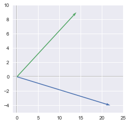
Note: we didn't include plt.show() in the function in order to be able to add plot configuration like here with the limits.

Note 2: we used the colors from seaborn manually with sns.color_palette()

So we have one error vector for each model. The better model is just the model corresponding to the smaller vector. One way to calculate the length of the vectors is to use the Pythagorean theorem: $\sqrt{x^2+y^2}$. We can calculate the length of the two vectors:

# Lenght of the vector errorModel1
np.sqrt(errorModel1[0]**2+errorModel1[1]**2)

22.360679774997898

# Lenght of the vector errorModel2
np.sqrt(errorModel2[0]**2+errorModel2[1]**2)

16.643316977093239

Congratulation! You just have calculated another norm of the error vectors. The length of the error vector of the first model is $22.36$ and the length of the error vector of the second model is around $16.64$. In this case, the second model is better but recall that we have just used the first two values.

We have first calculated the sum of the errors, but we can also use the Pythagorean theorem to compute the norm of a vector. These are two different norms, and it shows that there are multiple ways of calculating the norms.

Norm Functions: Definitions

The norm of a vector can be any function that maps a vector to a positive value. Different functions can be used, and we will see a few examples. These functions can be called norms if they are characterized by the following properties:

• Norms are non-negative values. If you think of the norms as a length, you can easily see why it can't be negative.

• Norms are $0$ if and only if the vector is a zero vector.

• Norms respect the triangle inequality. See below.

• $\norm{k\cdot \bs{u}}=\norm{k}\cdot\norm{\bs{u}}$. Here, $k$ is a scalar and $\bs{u}$ a vector. The norm of a vector multiplied by a scalar is equal to the absolute value of this scalar multiplied by the norm of the vector.

It is usually written with two horizontal bars: $\norm{\bs{x}}$

The Triangle Inequality

We have seen above that one condition for a function to be a norm is that it respects the triangle inequity. It just means that the norm of the sum of some vectors is less than or equal to the sum of the norms of these vectors:

Example 1.

To show what this means, we will take two vectors, each containing two elements (again, useful to be represented as x and y coordinates). Our vectors are:

u = np.array([1, 6])
u

array([1, 6])

and

v = np.array([4, 2])
v

array([4, 2])

Let's compare:

and:

We will see later different types of the norm, but for now on, we will use a classic one: the Euclidean Norm ($L^2$). The $L^2$ norm can be calculated with the Numpy function np.linalg.norm() (see more details on the doc).

We will see later in details what is the $L^1$ or $L^2$ norms.

np.linalg.norm(u+v)

9.4339811320566032

and

np.linalg.norm(u)+np.linalg.norm(v)

10.554898485297798

We can see that the triangle inequality is respected since:

Graphical explanation

You will see that the graphical representation of this theorem makes it quite trivial. We will plot the vectors $\bs{u}$, $\bs{v}$ and $\bs{u}+\bs{v}$ using our plotVectors function and adding some text to identify the vectors:

u = np.array([0,0,1,6])
v = np.array([0,0,4,2])
w = u+v

u_bis = [u[2], u[3], v[2], v[3]]

plotVectors([u, u_bis, w],
            [sns.color_palette()[0],
            sns.color_palette()[1],
            sns.color_palette()[2]])

plt.xlim(-2, 6)
plt.ylim(-2, 9)

plt.text(-1, 3.5, r'$||\vec{u}||$', color=sns.color_palette()[0], size=20)
plt.text(2.5, 7.5, r'$||\vec{v}||$', color=sns.color_palette()[1], size=20)
plt.text(2, 2, r'$||\vec{u}+\vec{v}||$', color=sns.color_palette()[2], size=20)

plt.show()
plt.close()

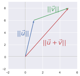
The length of $\bs{u}$ plus the length of $\bs{v}$ is larger than the length of the vector $\bs{u}+\bs{b}$. Geometrically, this simply means that the shortest path between two points is a line!

P-norms: General Rules

We have seen the conditions required by the function to be called norm. This means that there are multiple functions that can be used as norms. We will see later the pros and cons of these different norms. We call $p$-norm the following category of functions that depend on $p$:

Let's dive into this equation step by step. We can see that there is a sum of elements so we can think of it as an iteration over the $i$ elements:

1. $\vert\bs{x}_i\vert$ Calculate the absolute value of the $i$th element
2. $\vert\bs{x}_i\vert^p$ Take its power $p$
3. $\sum_i\vert\bs{x}_i\vert^p$ Sum all these powered absolute values
4. $(\sum_i\vert\bs{x}_i\vert^p)^{1/p}$ Take the power $\frac{1}{p}$ of this result

This will be clear with examples using these widely used $p$-norms.

The $L^0$ norm

If $p=0$, the formula becomes:

Let's see what it means. Using the power $0$ with absolute values will get you a $1$ for every non-$0$ values and a $0$ for $0$.

Therefore this norm corresponds to the number of non-zero elements in the vector. It is not really a norm because if you multiply the vector by $\alpha$, this number is the same (rule 4 above).

The $L^1$ norm

If $p=1$, we simply have the sum of the absolute values. It is what we have used intuitively at the beginning of this tutorial:

The $L^2$ norm (Euclidean norm)

The Euclidean norm is the $p$-norm with $p=2$. This may be the more used norm with the squared $L^2$ norm (see below).

We can note that the absolute value is not needed anymore since $x$ is squared. It is what we had used when we calculated the length of our vectors with the Pythagorean theorem above.

Let's see another example of this norm:

Example 2.

Graphically, the Euclidean norm corresponds to the length of the vector from the origin to the point obtained by linear combination (Pythagorean theorem). We will see an example in 2 dimensions: the vector $\bs{u}$ has two values corresponding to the $x$-coordinate and the $y$-coordinate. If you plot the point with these coordinates and draw a vector from the origin to this point, the $L^2$ norm will be the length of this vector.

For instance:

Let's start by calculating the norm with the formula:

So the $L^2$ norm is $5$.

By the way, remind that the $L^2$ norm can be calculated with the linalg.norm() function from Numpy:

np.linalg.norm([3, 4])

5.0

Here is the graphical representation of the vector:

u = np.array([3, 4])

plt.ylim(-1, 5)
plt.xlim(-1, 5)
plotVectors([u], [sns.color_palette()[0]])

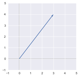
We can see that the vector goes from the origin (0, 0) to (3, 4) and that its length is 5.

In this case, the vector is in a 2-dimensional space, but this also stands for more dimensions.

The squared Euclidean norm (squared $L^2$ norm)

The squared $L^2$ norm is convenient because it removes the square root and we end up with the simple sum of every squared value of the vector.

The squared Euclidean norm is widely used in machine learning partly because it can be calculated with the vector operation $\bs{x}^\text{T}\bs{x}$. There can be performance gain due to optimization. See here and here for more details.

Example 3.

We will see in this example that the squared Euclidean norm can be calculated with vectorized operations. Let's start with a vector $\bs{x}$:

As usual, we will use code to check the process. First, let's create our Numpy vector $\bs{x}$:

x = np.array([[2], [5], [3], [3]])
x

array([[2],
       [5],
       [3],
       [3]])

Now let's take the transpose of this vector. This will just convert the initial column vector to a row vector:

We can calculate the transpose of $\bs{x}$ with the T method of Numpy objects:

x.T

array([[2, 5, 3, 3]])

The dot product of $\bs{x}$ and $\bs{x}^\text{T}$ (see here if you need some reminder about the dot product) corresponds actually to the multiplication of each element by itself:

This is exactly the definition of the squared Euclidean norm!

Let's check with Numpy. Remember (and try it to convince yourself) that the order the vector in the dot product matters:

euclideanNorm = x.T.dot(x)
euclideanNorm

array([[47]])

It should be our squared Euclidean norm! Let's calculate it from the $L^2$ norm and square it to check that this is right:

np.linalg.norm(x)**2

47.0

It works! The possibility to use a vectorized operation is a huge advantage over the other norms.

Derivative of the squared $L^2$ norm

We have seen that the norms can be used to evaluate the goodness of a model by summarizing the vectors of errors.

Now we want to go a step further and know how we can change the parameters of our model to reduce the overall error. To do that we can use a cost function that associates the error of the model in function of the parameters values. The gradient descent algorithm can be used to find the minimum of this function. The gradient descent is done by calculating the derivatives according to each parameter (partial derivatives = gradients). This is why this is crucial to be able to calculate the derivative efficiently.

Indeed, a big advantage of the squared $L^2$ norm is that its partial derivative is easily computed. Let's have the following vector:

We have seen that its squared $L^2$ norm is calculated with:

Then, to calculate the partial derivatives, we consider all other variables as constant. For instance, the partial derivative according to $u_1$ is the derivative of $u_1^2+a$ ($a$ being the constant corresponding to all other variables). For this reason, we have the following partial derivatives:

What is great about the gradients of the squared $L^2$ norm is that the derivatives do not depend on the other variables. We will see that it is not the case with the $L^2$ norm.

Derivative of the $L^2$ norm

In the case of the $L^2$ norm, the derivative is more complicated and takes every element of the vector into account. Let's take the last vector $\bs{u}$ as an example. The $L^2$ norm is:

Let's calculate the derivative of it according to $u_1$:

We can see that the partial derivative of $u_1$ still contains $u_2...u_n$. The other gradients follow the same structure:

Other considerations

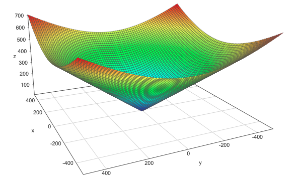
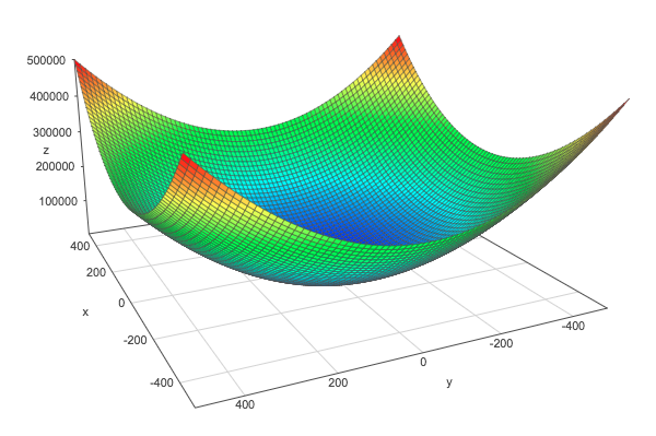
The squared $L^2$ norm is great, but one problem with it is that it hardly discriminates between 0 and small values because the function increases slowly.

We can see this by graphically comparing the squared $L^2$ norm with the $L^2$ norm. The $z$-axis corresponds to the value of the norm and the $x$- and $y$-axis corresponds to two parameters. The same thing is true with more than 2 dimensions, but it would be hard to visualize it.

$L^2$ norm:

Squared $L^2$ norm:

For comparison, here is the $L^1$ norm:

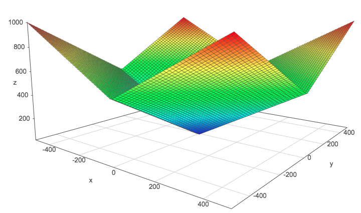
These plots have been done with the help of this website. Go and plot these norms if you need to move them in order to catch their shape.

The max norm

It is the $L^\infty$ norm and corresponds to the absolute value of the greatest element of the vector.

Matrix norms: the Frobenius norm

This is equivalent to take the $L^2$ norm of the matrix after flattening.

The same Numpy function can be used:

A = np.array([[1, 2], [6, 4], [3, 2]])
A

array([[1, 2],
       [6, 4],
       [3, 2]])

np.linalg.norm(A)

8.3666002653407556

Expression of the dot product with norms

The dot product between the vectors $\bs{x}$ and $\bs{y}$ can be retrieved with the $L^2$ norms of these vectors. $\theta$ is the angle between the two vectors.

Example 4.

Let's take two vectors in 2 dimensions:

and

The following plot shows their graphical representation:

x = [0,0,0,2]
y = [0,0,2,2]

plotVectors([x, y], [sns.color_palette()[0], sns.color_palette()[1]])

plt.xlim(-1, 3)
plt.ylim(-1, 3)

plt.text(-0.5, 1, r'$\vec{x}$', size=18, color=sns.color_palette()[0])
plt.text(1.5, 0.5, r'$\vec{y}$', size=18, color=sns.color_palette()[1])

<matplotlib.text.Text at 0x10a33b950>

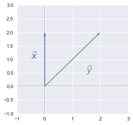
We took this example for its simplicity. As we can see, the angle $\theta$ is equal to 45°.

First, let's calculate the dot product of the vectors:

x = np.array([0, 2])
y = np.array([2, 2])

x.dot(y)

4

And now let's calculate their norms:

and

So with the above formula, we have:

This is the same results as with the dot product. Here are the operations using numpy. Just note that we use the function deg2rad from Numpy because np.cos takes the angle in radian, so we have to do the conversion.

# Note: np.cos take the angle in radian
np.cos(np.deg2rad(45))*2*np.sqrt(8)

4.0000000000000009

Conclusion

The $L^2$ norm (or the Frobenius norm in case of a matrix) and the squared $L^2$ norm are widely used in machine learning, deep learning and data science in general. For example, norms can be used as cost functions. Let's say that you want to fit a line to a set of data points. One way to find the better line is to start with random parameters and iterate by minimizing the cost function. The cost function is a function that represents the error of your model, so you want this error to be as small as possible. Norms are useful here because it gives you a way of measuring this error. The norm will map the vector containing all your errors to a simple scalar, and the cost function is this scalar for a set of value for your parameters.

We have seen that norms are nothing more than an array reduced to a scalar. We have also noticed that there are some variations according to the function we can use to calculate it. Choosing which norm to use depends a lot of the problem to be solved since there are some pros and cons for applying one or another. For instance, the $L^1$ norm is more robust than the $L^2$ norm. This means that the $L^2$ norm is more sensible to outliers since significant error values will give enormous squared error values.

This tutorial is based on this article from my series about the linear algebra chapter in the Deep Learning Book by Goodfellow et al.

References

https://www.quora.com/Why-is-L1-regularization-better-than-L2-regularization-provided-that-all-Norms-are-equivalent

http://www.deeplearningbook.org/contents/linear_algebra.html

https://docs.scipy.org/doc/numpy-1.14.0/reference/generated/numpy.linalg.norm.html

https://hadrienj.github.io/deep-learning-book-series-home/

http://christopher5106.github.io/deep/learning/2016/09/16/about-loss-functions-multinomial-logistic-logarithm-cross-entropy-square-errors-euclidian-absolute-frobenius-hinge.html

https://datascience.stackexchange.com/questions/10188/why-do-cost-functions-use-the-square-error